

K-means clustering algorithm from scratch
Matlab project.
K-means algorithm classes n observations into k clusters in which each observation belongs to the nearest cluster.
GitHub link: https://github.com/Apiquet/KMEANS_algorithm
1- K-means explanation through an example
As it’s always easier to understand through an example, let’s see the following one:
Imagine a 2D-dataset composed by 9 data points:
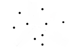
Then, applying a K-means algorithm with K equals to 3 would give the following result:
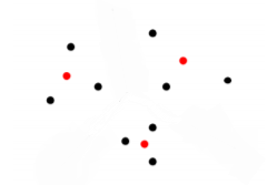
Each cluster took an average value of several data points. The following classification is performed:

Now, all the data points are relied to a cluster.
In the following part, we will compress an image with this method.
2 – Influence of K in image compression/reconstruction
2.1- Compression
To understand the influence of K, imagine that each data point (in the example above) represents a pixel in an image. An image of 3×3 pixels. Each pixel has a specific color. With a K-means process with K=3, we will create 3 new pixels that represents an average of several real pixels. Then we will save for each data point, which cluster is the closest. So, at the end of the K-means process we will only have 3 pixels in memory and a table with one number for each pixel that represents its closest cluster’s number.
2.2- Reconstruction
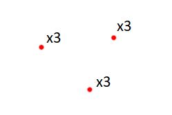
To reconstruct the image from that data, we will create 9 pixels (the number of row in the table) with the associated clusters. In our example, we will create 9 pixels with 3 different values (3 with the cluster 1, 3 with the cluster 2 and 3 with the cluster 3).
The result would be:
2.3- Influence of K
We lose nuances in the process but the data is lighter in memory. However, the higher the K, the less nuances are lost! But the higher the K, the more memory the compressed image will take.
3- How to implement a K-means algorithm
3.1- Distance calculation
We first need to implement a function to get the distance between the data points. To achieve that we have several solutions:
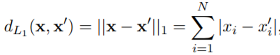
switch type
case 'L1' % Manhattan Distance
for i=1:N
d=d+abs(x_1(i)-x_2(i));
end
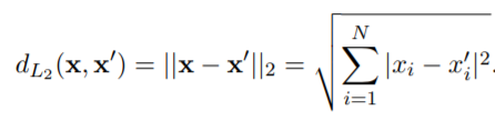
case 'L2' % Euclidean Distance
for i=1:N
d=d+(abs(x_1(i)-x_2(i)))^2;
end
d=sqrt(d);
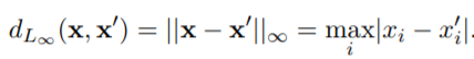
case 'LInf' % Infinity Norm
absDiff = abs( x_1 - x_2 ) ;
d = max( absDiff ) ;
end
3.2- Initializing K-means algorithm
To start implementing the K-means algorithm, we need to initialize a matrix Mu that has k columns that correspond to the k centroids. We can choose the k points randomly or uniformly:
if init == "random"
   for i=1:k
      index=randi([1 M]);
      Mu(:,i) = X(:,index);
   end
elseif init == "uniform"
   Mu(1,:) = datasample(X(1,:),k);
end
3.3- Implementing K-means algorithm
Our K-means algorithm will be composed of 3 main steps:
- assigning each point to its closest cluster centroids:
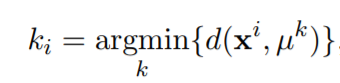
- getting the label of the closest cluster:
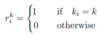
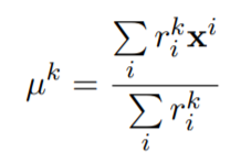
- recomputing the centroids:
%Equation 1
[~,labels] = min(d_i);

%Equatin 2
for i=1:K
   for j=1:M
      if (i==labels(j))
         r_i(i,j)=1;
      else
         r_i(i,j)=0;
      end
   end
end

%Equation 3
for j=1:K
   Multiplication_Matrix = zeros(N, K);
   Sum = 0;
   for i=1:M
      Multiplication_Matrix(:,j)=Multiplication_Matrix(:,j)+r_i(j,i).* X(:,i);
   end
   Sum=Sum+sum(r_i(j,:));
   Mu(:,j)=Multiplication_Matrix(:,j)/Sum;
end
4- Result on real image
To see the real impact of K, we need to apply our algorithm on a real image. The following images show the result for K equal to 3, 5 and 11. The first one is the original image:

The code is available on my Github repository:
