

State of the Art: Object detection (1/2)
The aim of this article is to give a state of the art of object detection evaluated on COCO and classified by architecture type. Then, the transformers will be explained starting from the NLP domain to their adaptation to the computer vision domain with the Swin Transformers and the Focal Transformers. The methods presented in the SwinV2-G paper to adapt the Swin Transformer to a 3 billion parameters model will also be explained.
Table of contents
- State-of-the-art: Object detection
- Metrics
- box AP
- FLOPs / FLOPS / MACs
- Ranking
- Swin Transformers
- Focal Transformers
- YOLOR
- ResNeXt: DETR, SOLQ, CenterNet2
- EfficientDet
- SSD
- Metrics
- Paper overview
- SwinV2-G
- Transformer
- Swin transformer
- Swin-T
- Methods
- HTC
- HTC++
- Techniques for scaling Swin Transformer
- Focal-L
- SwinV2-G
- Conclusion
1) State of the art
1-1) Metrics
1-1-1) Box ap
On the COCO results page, the Box AP metrics states for mAP which means the average results over several IoU thresholds starting from 0.5 to 0.95 with a step size of 0.05. This is calculated and averaged over 80 classes.
The AP metric for a specific IoU threshold is the area under the precision-recall curve calculated for confidences from 0.0 to 1.0.
A full description of this metric, with examples, can be found in the following article.
1-1-2) FLOPs / FLOPS / MACs
To measure the computational cost of an algorithm, we cannot use the number of FPS because it depends on the hardware used. To avoid to this problem, FLOPs (FLoating point OPerations) is used to calculate the number of operations needed to do a single inference.
As the number of operations can be very large, MFLOPs (10e6), GFLOPs (10e9) or TFLOPs (10e12) can be used.
This is not to be confused with the term FLOPS which stands for FLoating point OPerations per Second used to describe the performance of a hardware.
FLOPs calculation explanation can be found in this article and this one. The FLOPs for a convolution and a fully connected layer are:


Tools also exist to calculate the FLOPs of a model, for instance flop_count_operators from Detectron2
FLOPs of some well known architectures can be found here.
MACs (Multiply-Accumulate Computations) also exists. A MAC does an addition and a multiplication, so 1 MAC = 2 FLOPs.
MAC can also mean the Memory Access Cost that must be taken to complete FLOPs one. For example, although the computations required for addition or concatenation of branches are negligible, the MAC is significant.
1-2) Ranking
Actual ranking for object detection on COCO dataset can be found here and may differ from the one given bellow.
1-2-1) Swin Transformers
| Model | Global Ranking | mAP | Param | GFLOPs |
| SwinV2-G | 1 | 63.1 | 3B | >1470 |
| Florence-CoSwin-H | 2 | 62.4 | 893M | – |
| GLIP | 3 | 61.5 | – | – |
| Soft Teacher + Swin-L | 4 | 61.3 | – | – |
| DyHead | 5 | 60.6 | – | – |
| Dual-Swin-L | 6 | 60.1 | 453M | >836 |
| Swin-L | 10 | 58.7 | 284M | >1470 |
| Deformable DETR | 39 | 52.3 | >40M | >173 |
1-2-2) Focal Transformers
Model | Global Ranking | mAP | Param | GFLOPs |
| Focal-L (DyHead) | 10 | 58.9 | 229M | 1081 |
| Focal-L (HTC++) | 13 | 58.4 | 265M | 1165 |
1-2-3) YOLOR
| Model | Global Ranking | mAP | Param | GFLOPs |
| YOLOR-D6 | 13 | 57.3 | 152M | 936.8 |
1-2-4) ResNeXt
| Model | Global Ranking | mAP | Param | GFLOPs |
| CenterNet2 | 17 | 56.4 | – | – |
| DetectoRS | 20 | 55.7 | – | – |
| UniverseNet-20.08d | 29 | 54.1 | – | – |
| PAA | 31 | 53.5 | – | – |
| LSNet | 32 | 53.5 | – | – |
| ResNeSt-200 | 33 | 53.3 | – | – |
| CBNet on Cascade Mask R-CNN | 34 | 53.3 | – | – |
| GFLV2 | 36 | 53.3 | – | – |
| RelationNet++ | 37 | 52.7 | – | – |
| RepPoints v2 | 42 | 52.1 | 38M | 236 |
1-2-5) EfficientDet
| Model | Global Ranking | mAP | Param | GFLOPs |
| EfficientDet-D7x | – | 55.1 | 77M | 410 |
| EfficientDet-D7 | 30 | 53.7 | 52M | 325 |
| EfficientDet-D6 | – | 52.6 | 52M | 226 |
| EfficientDet-D5 | – | 51.5 | 34M | 135 |
| EfficientDet-D4 | – | 49.7 | 21M | 55 |
| EfficientDet-D3 | – | 47.2 | 12M | 25 |
| EfficientDet-D2 | – | 43.9 | 8.1M | 11 |
| EfficientDet-D1 | – | 40.5 | 6.6M | 6.1 |
| EfficientDet-D0 | – | 34.6 | 3.9M | 2.5 |
1-2-6) SSD
This architecture has been explained and implemented in Tensorflow in the following article.
2) Paper overview
An overview of many Object Detection models can be found here.
2-1) SwinV2-G
2-1-1) Transformer
A transformer uses the mechanism of self-attention to find the significance of each part of the input data. They are designed to handle sequential input data without the need to process the data in order. This feature allows for more parallelization than RNNs which needs the order.
Transformers are increasingly the model of choice for NLP problems. Their training parallelization allows the use of larger datasets, which led to the development of pretrained systems such as BERT (Bidirectional Encoder Representations from Transformers) and GPT (Generative Pre-trained Transformer).
2-1-1-a) Transformer in NLP
In the BERT architecture previously mentioned, a non-directional training of Transformer is used. This is opposed to the traditional approaches that train on a text sequence from left to right (or right to left).
A Transformer is composed of an encoder which reads the sequence of words (tokenized with vectors) and a decoder that outputs a prediction.
This transformer architecture was presented in the article “Attention is all you need” which indicates that this architecture, without recurrence or convolution, obtained state-of-the-art results on two machine translation tasks. This model is also more parallelizable, which significantly reduces the learning time.
Summary of the paper Attention is all you need:
The transformer consists of an encoder that transforms an input sequence (x1, …, xn) into a sequence of continuous representations z = (z1, …, zn) of continuous representations z = (z1, …, zn). Given z, the decoder then generates an output sequence (y1, …, ym) of symbols, one element at a time. At each step, the model is auto-regressive it uses the previously generated symbols as additional input when generating the next.
The illustration above shows the encoder (left) and the decoder (right).
The encoder is composed of a stack of N = 6 identical layers. Each layer has two
sub-layers:
- a multi-head self-attention mechanism,
- a positionwise fully connected feed-forward network.
A residual connection around each of the two sub-layers is used, followed by layer normalization. To facilitate these residual connections, all sub-layers in the model, as well as the embedding layers, produce outputs of dimension 512.
The decoder is also composed of a stack of N = 6 identical layers. In addition to the two sub-layers in each encoder layer, the decoder inserts a third sub-layer, which performs multi-head attention over the output of the encoder stack. Residual connections around each of the sub-layers are also used, followed by layer normalization. The self-attention sub-layer is modified to prevent positions from attending to subsequent positions. This masking, combined with fact that the output embeddings are offset by one position, ensures that the predictions for position i can depend only on the known outputs at positions less than i.
The Multi-Head Attention runs several Attention layers in parallel. An Attention function can be described as mapping a query and a set of key-value pairs to an output, where the query, keys, values, and output are all vectors. The output is computed as a weighted sum of the values, where the weight assigned to each value is computed by a compatibility function of the query with the corresponding key:

The Scaled Dot-Product Attention takes as input queries and keys of the same dimension, computes the dot products and scale each element by 1/sqrt(dimension). A Softmax function is then applied to get the weights to multiply with the input values. The final computation is:

This attention module differs from those commonly used:
- Dot-product attention: does not have the scale layer with factor 1/sqrt(dimension)
- Additive attention: computes the compatibility function with a feed-forward network with one hidden layer
Note: dot-product attention is faster and more space-efficient thanks to optimized matrix multiplication code.
The addition of scaling counteracts the side effect of a large dimension value. Indeed, additive attention and dot-product have similar performance for small dimensions, but for larger values, the dot-product seems to suffer from small gradients. This seems to be caused by a large magnitude pushing the softmax function into regions where gradients are small.
The Multi-Head Attention learns linear projections of queries, keys and values on which the Attention module is applied on parallel. The Multi-Head’s results are then concatenated, and once again projected to get the final results:

Mask: self-attention layers in the decoder allow each position in the decoder to attend to all positions in the decoder up to and including that position. To preserve the auto-regressive property, the leftward information flow in the decoder should be avoided. This is implemented inside of scaled dot-product attention by masking out (setting to −∞) all values in the input of the softmax which correspond to illegal connections.
Position-wise Feed-Forward Network: the Feed-Forward parts of the architecture are composed of two linear transformations applied in sequence, the first one with a ReLU activation.
Embeddings: learned embeddings are used to convert the input and output tokens to vectors. The same weight matrix is shared between the two embedding layers. This weights are multiplied by sqrt(model dimension).
Positional encoding: it allows to use the relative or absolute position of the token in a given sequence. This must be done because there is no recurrence or convolution. This positional encoding is of the same dimension as the embeddings, they are added. This encoding can be learned or fixed. In this paper, sine and cosine functions of different frequencies are used:
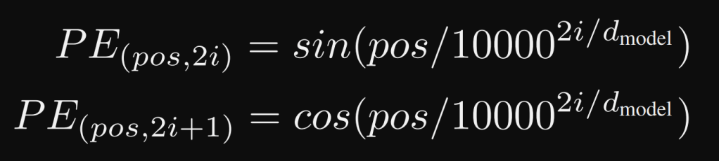
where pos is the position and i the dimension. Learned positional embeddings where also tried and give similar results. This article explains why sin and cos are used.
For a more in-depth understanding of transformers/self-attention, please refer to this and this articles.
2-1-1-b) Transformer in Computer Vision
In the field of computer vision, convolutions are widely used. A convolution extracts features with a learned kernel, which has a specific receptive field. This allows convolutions to be translation invariant (they find the learned feature anywhere in the input) and locally sensitive (restricted to the receptive field).
To learn the dependencies between objects in an image, convolutions must increase their receptive field. To do this, we can use larger kernels, dilated convolutions, a cascade of many convolutions with decreased spatial resolution (using dilation, stride, pooling, etc.). However, this is not done without loss of efficiency, it can also create models that are very difficult or impossible to train.
As with NLP tasks, transformers/self-attention arrived in the field of computer vision to solve the problem of lack of global image understanding that convolutions suffer from.
These transformers can be applied:
- alone, without the need for convolutions (transformers can behave similarly to a convolution),
- using a backbone of convolutions, then transformers. In this case, the transformers compute the attention weights between the features. They can take as input:
- Flattened features: [WxH, F], with W: width, H: height, F: depth,
- Features [W, H, F] and compute along the width then the height,
- Patched features that reduce the receptive field but remain much larger than those of the convolutions.
In the next section, we will delve into the implementation of transformers for computer vision tasks. This will be done through the explanation of the article on Image Transformers.
Summary of the paper Image Transformer:
This work showed how Transformers can be applied to computer vision tasks. On image generation, their model significantly outperformed the current SOTA on ImageNet. They also implemented an encoder-decoder configuration of their architecture for image super-resolution. In a human evaluation study, they found that images generated by their super-resolution model fool human observers three times more often than the previous SOTA models.
Even though transformers are used for images, many aspects are very similar to those seen previously for NLP. The paper gives an illustration of a slice of an Image Transformer layer:
This layer is used to compute the new representation of q, named q’. To do so, the attention layer takes into account the vector M of the previously generated pixels, which are added with a vector of position encodings.
As discussed in the previous article, Attention Is All You Need, they evaluated two different coordinate encodings: sine and cosine functions of coordinates, with different frequencies and learned position embeddings.
Then a projection with key and value matrices is performed, as in the previous section. Finally, a dropout has been added.
The end of the layer is also very similar to the previous section:
A Softmax function is also used on a dot scalar product also divided by sqrt(dimension). Finally, a layer normalization is applied on a Position-Wise Feed Forward Network to compute a linear projection on another linear projection activated with a ReLU function (also performed in the previous paper in NLP).
Now that we are familiar with transformers, the next section will delve into the SwinV2-G architecture by explaining the Swin transformer concept.
2-1-2) Swin Transformer
This section will base its explanations on the Swin Transformer paper.
They proposed a hierarchical transformer whose representation is computed with staggered windows. The staggered windowing scheme provides greater efficiency by restricting the computation of self-attention to non-overlapping local windows while allowing for connection between windows.
This hierarchical architecture has the flexibility to model at various scales and has linear computational complexity with respect to image size. These qualities of Swin Transformer make it compatible with a broad range of vision tasks, including image classification and dense prediction tasks such as object detection and semantic segmentation.
The authors want to address two main problems researchers face in transferring transformers from the language domain to the vision domain:
- Scale: Unlike word tokens, visual elements can vary considerably in scale, a problem that gets attention in tasks such as object detection. In existing transformer-based models, the tokens all have a fixed scale,
- Computational problem caused by the much higher resolution of pixels in images compared to words in text passages.
As shown in the figure legend above, their proposed method achieves linear computational complexity instead of quadratic complexity. To do this, instead of computing self-attention globally (on each pixel), they compute it on a fixed number of patches in each window:
Window based MSA (W-MSA) linear complexity with image size
The Swin transformer implements a “window partition shift” between consecutive self-attention layers. These shifted windows link the previous layer’s windows, providing connections between them that greatly improve modeling power :
They also improved the latency of previous architectures that used sliding windows by using the same set of keys on a query patch.
However, this technique has two issues:
- it increases the number of patches for the layer l+1
- it creates patches of non-uniform sizes
The authors indicate that a naive solution could be to pad each small patch to a uniform size, but this significantly increases the processing time. They propose a new method called “cyclic-shifting” which is illustrated as follows:
The problematic parts A/B/C are translated into other parts to create patches of uniform size. Then, a masking is used to allow, for example, the pixels in B to depend only on the pixels in B. We can note that masking was also used in NLP to avoid the leftward information flow in the decoder to preserve the auto-regressive property.
They also added a relative position bias to each head, which increases performance:
Their architecture exists in several forms:
The base model, called Swin-B, has a size and a computation complexity similar to ViTB/DeiT-B. Swin-T, Swin-S and Swin-L, are versions of about 0.25×, 0.5× and 2× the base model size and computational complexity, respectively. The architecture hyper-parameters of these model variants are:
2-1-2-1) Swin-T
Swin-T is for the Tiny version of the Swin Transformer:
Stage 1: splits input RGB image into non-overlapping patches, like ViT. Each patch is treated as a “token” and its feature is set as a concatenation of the raw pixel RGB values. A patch size of 4×4 is used and thus the feature dimension of each patch is 4×4×3=48. A linear embedding layer is applied on this raw-valued feature to project it to an arbitrary dimension (denoted as C)
Stage 2: to produce a hierarchical representation, the number of tokens is reduced by patch merging layers as the network gets deeper. The first patch merging layer concatenates the features of each group of 2×2 neighboring patches, and applies a linear layer on the 4C-dimensional concatenated features. This reduces the number of tokens by a multiple of 2×2 = 4 (2× downsampling of resolution), and the output dimension is set to 2C. Swin Transformer blocks are applied afterwards for feature transformation, with the resolution kept at H/8 × W/8.
Stage 3-4: the procedure is repeated twice with output resolutions of H/16 × W/16 and H/32 × W/32.
A Swin Transformer block consists of a shifted window based MSA module, followed by a 2-layer MLP with GELU nonlinearity in between (instead of ReLU seen in previous papers). A LayerNorm (LN) layer is applied before each MSA module and each MLP, and a residual connection is applied after each module.
2-1-3) Methods
2-1-3-1) HTC
In their paper, the authors explored more effective approaches of Cascade Mask R-CNN (detailed on the next article). They found that the key to a successful instance segmentation cascade is to fully leverage the reciprocal relationship between detection and segmentation. The Hybrid Task Cascade (HTC), differs in two important aspects: (1) instead of performing cascaded refinement on these two tasks separately, it interweaves them for a joint multi-stage processing; (2) it adopts a fully convolutional branch to provide spatial context, which can help distinguishing hard foreground from cluttered background.
They improved the Cascade Mask R-CNN in 4 main steps illustrated in the following figure:

- b) the mask branch can take advantage of the updated bounding box predictions,
- c) information flow between mask branches by feeding the mask features of the preceding stage to the current stage,
- d) (HTC) to further help distinguishing the foreground from the cluttered background, they used the spatial contexts as an effective cue. They added an additional branch to predict per-pixel semantic segmentation for the whole image, which adopts the fully convolutional architecture and is jointly trained with other branches.
The semantic segmentation branch S is constructed based on the output of the Feature Pyramid:
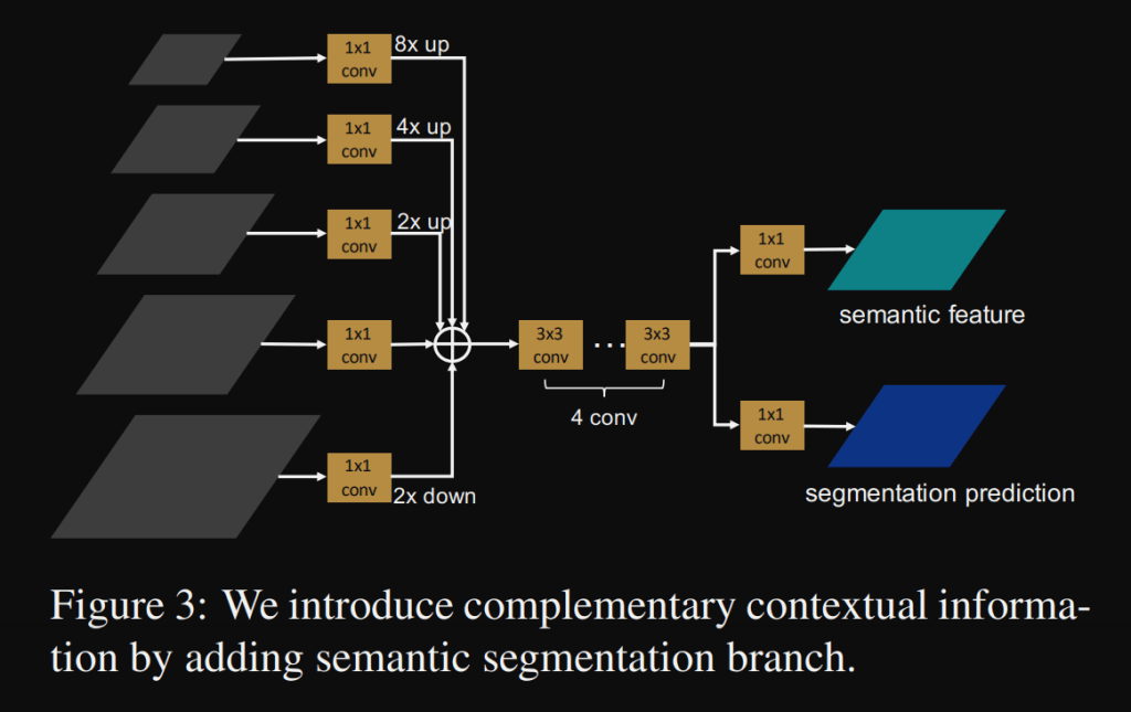
Each level of the feature pyramid is first aligned to a common representation space via a 1 × 1 convolutional layer. Then low level feature maps are upsampled, and high level feature maps are downsampled to the same spatial scale, where the stride is set to 8.
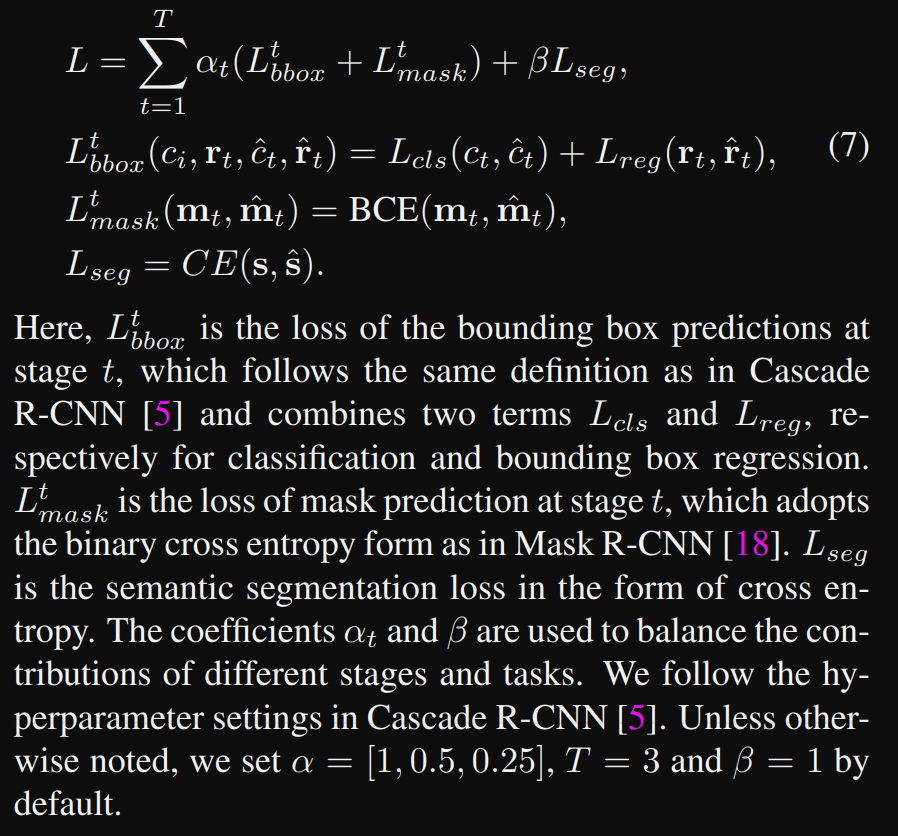
All the modules described above are differentiable, Hybrid Task Cascade (HTC) can be trained in an end-to-end manner. At each stage t, the box head predicts the classification score ct and regression offset rt for all sampled RoIs.
The mask head predicts pixel-wise masks mt for positive RoIs. The semantic branch predicts a full image semantic segmentation map s. The overall loss function takes the form of a multi-task learning:
An improved version of HTC (named HTC++) was used in the Swin Transformer.
2-1-3-2) HTC++
In the Swin Transformer paper, the authors adopted an improved HTC (denoted as HTC++) with instaboost (method to augment the training set using the existing instance mask annotations), stronger multi-scale training, 6x schedule (72 epochs), soft-NMS, and ImageNet-22K pre-trained model as initialization.
2-1-4) Techniques for scaling Swin Transformer
In the SwinV2-G model, the authors present techniques for scaling Swin Transformer up to 3 billion parameters and making it capable of training with images of up to 1,536×1,536 resolution. Their techniques are summarized in the first figure of the paper:
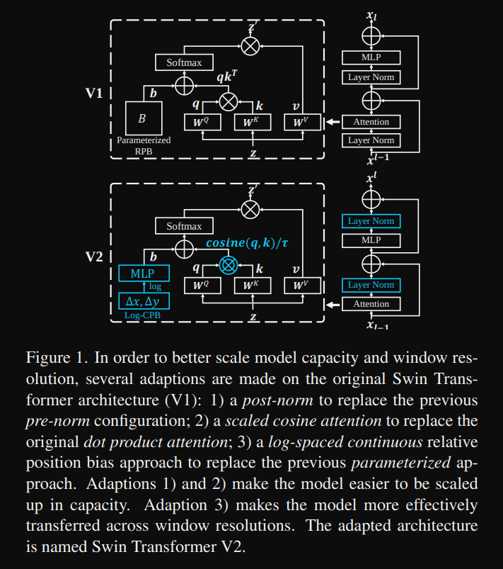
They found that the gap in activation amplitudes between layers becomes significantly larger in large models. A closer look at the original architecture reveals that this is due to the fact that the output of the residual unit is directly added to the main branch. As a result, the activation values are accumulated layer by layer, and thus the amplitudes of the deepest layers are significantly larger than those of the first layers. To address this problem, they propose a new normalization configuration, called post-norm, which moves the LN layer from the beginning of each residual unit to the back end.
They also proposed a scaled cosine attention to replace the previous dot product attention. The scaled cosine attention makes the computation irrelevant to amplitudes of block inputs, and the attention values are less likely to fall into extremes.
Many downstream vision tasks, such as object detection and semantic segmentation, require high-resolution input images or large attention windows. Variations in window size between low-resolution pre-training and high-resolution fine-tuning can be quite large. The common practice is to perform bi-cubic interpolation of the position bias maps. This simple solution is somewhat ad-hoc and the result is usually suboptimal. They introduced a log-spaced continuous position bias (Log-CPB), which generates bias values for arbitrary coordinate ranges by applying a small meta-network to the log-spaced coordinate inputs. Since the meta-network takes any coordinates, a pre-trained model will be able to be freely transferred from one window size to another by sharing the meta-network weights.
The scaling up of model capacity and resolution also leads to prohibitively high GPU memory consumption. To resolve the memory issue, they incorporated several important techniques: zero-optimizer, activation check pointing and a novel implementation of sequential self- attention computation:
- Zero-optimizer: described here, is a new parallelized optimizer that greatly reduces the resources needed for model and data parallelism while massively increasing the number of parameters that can be trained,
- Activation check pointing: described here, reduces the memory cost to store the intermediate feature maps and gradients during training,
- Sequential self- attention computation: implements the self-attention computation sequentially, instead of using the previous batch computation approach. This optimization is applied on layers in the first two stages.
They also added larger configurations of the Swin Transformers seen previously:

2-2) Focal-L
In this paper, the authors present focal self-attention, a new mechanism that incorporates both fine-grained local and coarse-grained global interactions. In this new mechanism, each token attends its closest surrounding tokens at fine granularity and the tokens far away at coarse granularity, and thus can capture both short- and long-range visual dependencies efficiently and effectively.
They proposed a new variant of Vision Transformer models, called Focal Transformer. They present a new self-attention mechanism to capture both local and global interactions in Transformer layers for high-resolution inputs. Considering that the visual dependencies between regions nearby are usually stronger than those far away, they perform the fine-grained self-attention only in local regions while the coarse-grained attentions globally:


Model architecture:

Patch embedding: convolutional layer with filter size and stride both equal to 4, to project these patches into hidden features with dimension d.
Focal Self-Attention at window level:

They also implemented several configurations from Tiny to Large, with the same design saw in the Swin Transformer paper (section 1-2-1). Here is a summary for the configurations Tiny, Small and Base:

Conclusion
Transformers were first developed in NLP and quickly showed their advantages over RNNs: (1) the data does not have to be fed in sequence, which allows for greater parallelism, (2) a self-attention mechanism is used to compute the similarity between words (long and short term).
These transformers have also been adapted to the field of computer vision and allow for a better overall understanding of the input due to their larger receptive fields. It has also been shown that the transformers behave like a convolution at the first stages and allows the model to consist of only transformers.
We can also mentioned that the first 14 models of the COCO ranking are models based on Transformers.
The next article will give an overview of other methods: YOLOR, CBNet, R-CNN series, CenterNet, DetectoRS and EfficientDet.
