AI, Java

Maximizing delivery profit thanks to AI

JAVA project.

Thanks to some famous AI algorithms, we will maximize the delivery profit of a Switzerland company.

GitHub link: https://github.com/Apiquet/AI_DeliberativeAgents

To achieve this goal we will use Repast J software to build a simulation. We will implement several types of delivery drivers to compare different AI algorithms’ performance.

The Breadth-first search and A* algorithms will be explained and implemented in this article.

Table of contents

1. The context
2. The model.
   1. Intermediate States
   2. Goal State
   3. Actions
3. Implementation
   1. BFS
   2. A*
   3. Heuristic Function
4. Results
   1. Experiment 1: BFS and A* Comparison
   2. Experiment 2: Multi-agent Experiments

1) The context.

In the simulation, delivery drivers have to take care of packages. Each package must be picked up in one city and delivered in another. In addition, each task has a weight and each delivery driver has a maximum weight he can carry.

We will set up three drivers, a normal one that takes each packet one by one, a BFS driver and an A* driver. Then we will compare the results. Since we set the number of packages and the rewards, the goal here is to minimize the cost (the number of km done to deliver all the tasks).

2) The model.

2.1) Intermediate States

In order to implement the algorithms, we need to define the characteristics of a state. Typically, we needed the list of packets that need to be delivered and information about the transported task. We chose a HashTable, the packet as key and a boolean value as value (true if we should take the packet, otherwise false).

The packet is removed from the HashTable when we deliver it. Then, we need the current space available in the truck, the current city, the current cost and the list of actions to reach the current state (in order to build the optimal plan at the end).

2.2) Goal State

The goal state is simply a state with an empty HashTable because we remove a packet when it was delivered. Our tree is composed of multiple states with a number of packet to pick up and/or deliver, this list decreases each time we deliver a packet until it is empty.

2.3) Actions

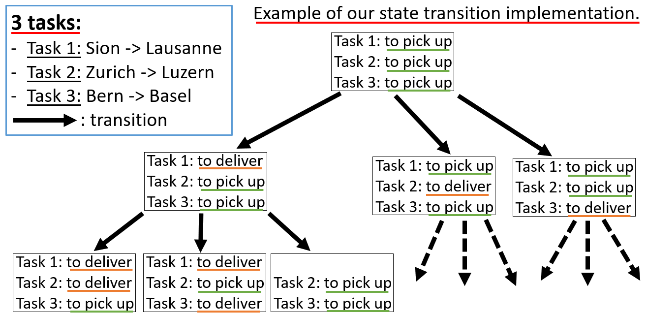
The actions are: moving to a city with a task to pick up or deliver.

With this implementation, if we have three tasks to pick up, we will get three new states from the initial state. Here a representation of our state transition:

3) Implementation

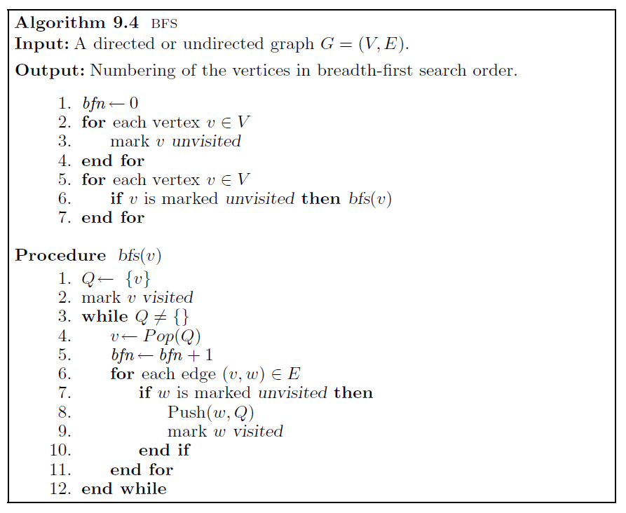
3.1) BFS

The BFS implementation must compute the entire tree (see Figure 1) to find the optimal plan with the minimum cost. This computation is expensive in terms of memory and resources. To perform this algorithm, a list of states that represents the last level of the tree is computed. In other words, in the example of figure 1, the initial size of the state list is 1, then 3, then 9, then 24 (because 3 states among the 9 have only 2 packets), etc. Since each state has the list of actions needed to compute its plan and cost, we only need the last level of the tree to compare the plans and compute the best one. This implementation frees the memory of all previous states.

The algorithm from www.chegg.com:

To implement this algorithm in Java we will use some specific objects like HashTable, ArrayList, and we will need to define some classes.

Classes will be used for States and Action, ArrayList the actions and states history.

ArrayList action_list = new ArrayList();
ArrayList state_list = new ArrayList();
Hashtable task_table = new Hashtable();

Then, the loop need to be implemented to calculate each state. Typically, for each state, we calculate the next possible ones. In other word, if I’m in a state with 2 packets that need to be picked up, my next possible states would be: 1- A state with the task 1 picked up, 2- A state with the task 2 picked up.

while(!state_list.isEmpty()) {
   for(int i=0;i<state_list.size();i++) {
      for (Entry entry : state_list.get(i).task_table.entrySet()) {
         State newState = state_list.get(i).clone();
         City final_City = newState.getCurrentCity();
         if(entry.getValue() == true && entry.getKey().weight  pickup location
         for (City city : newState.getCurrentCity().pathTo(entry.getKey().pickupCity)) {
            final_City = moveTo(city);
         }
         pickupTask(entry.getKey());
      }
      else if(entry.getValue() == false) {
         // move: pickup location => delivery location
         for (City city : newState.getCurrentCity().pathTo(entry.getKey().deliveryCity)) {
            final_City = moveTo(city);
         }
         deliverTask(entry.getKey());
      }
      else continue;
      if(newState.task_table.isEmpty()) finalstate_list_bfs.add(newState);
      else state_list.add(newState);
      }
   }
}
//finding best action
ArrayList bestActionList = FindBestState(finalstate_list_bfs);
Plan plan = new Plan(vehicle.getCurrentCity());
//building best plan with best action list
plan=BuildingPlan(vehicle.getCurrentCity(), plan, bestActionList);
return plan;

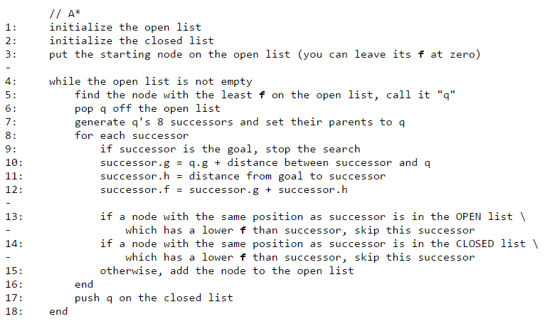
3.2) A*

The A* implementation does not need to compute the whole tree. We only need to find a pseudo-optimal (close to the true optimal) plan faster. To achieve this, we observe the next possible states for each state we just computed, and then keep only the states that lead to the minimum cost states. An alpha number determines how far we will observe in a heuristic function.

The objective is based on the cost of the trip which must be minimized.

Here the algorithm from https://stackoverflow.com:

3.3) Heuristic Function

Thanks to an alpha number, we choose how far we will predict the next states’ cost.

With alpha equals to 1, we would calculate the level 2 with 3 states, then we will do a prediction of the next 9 states (each one will lead to a specific cost). We will only keep the state (of the 3 states) that has the minimal cost for the next level. As it’s easier to explain thanks to an example, you can see the Figure 2:

If we compute the A* algorithm with alpha=1, we will remove ”State 1”, if we choose alpha=2, we will remove the ”State 2”. Afterwards, we will recompute that system with ”State 1” or ”State 2” as ”initial State”.

To implement this function we need to star from the BFS algorithm. The main difference is to avoid calculating the entire tree. Our alpha number will determine how far we will calculate. We just need to add a for loop to process the BFS algorithm alpha times, Then took the best state as defined by my example above.

while(finalstate_list_astar.isEmpty()) {
   for(int j=0;j<alpha;j++) {
      BFS_algorithm(action_list,state_list,task_table);
   }
   if(!state_list.isEmpty() && !planCancelled) {
      State minimalCostState = new State();
      int indexStateMinCost = -1;
      int minCost=Integer.MAX_VALUE;
      for(int i=0;i<state_list.size();i++) {
         if(state_list.get(i).getCost()<minCost) {
            minCost=state_list.get(i).getCost();
            indexStateMinCost=state_list.get(i).getIdentity();
         }
      }
      for(int i=0;i<transition_state_list.size();i++) {
         if(transition_state_list.get(i).getIdentity()==indexStateMinCost) {
            minimalCostState=transition_state_list.get(i);
            break;
         }
      }
      state_list.clear();
      transition_state_list.clear();
      state_list.add(minimalCostState);
   }
}

4) Results

4.1) Experiment 1: BFS and A* Comparison

First, the BFS algorithm always find the optimal plan, that’s a good point. However, its calculation is very costly and its cost is exponential with the number of packets. Second, the A* algorithm also find the optimal plan if there are less than 7 packets. However, it is much less costly.

Example of simulation with 7 tasks to pick up and one driver:

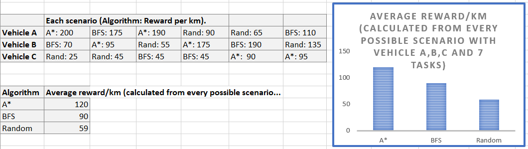
4.2) Experiment 2: Multi-agent Experiments

The result was better than expected. A* algorithm got an average of 120 reward per km. The BFS algorithm got 90 so 25% less and the random one got 59 so 50% less than A* and 34% less than BFS.

Here an example of multi agents simulation:

The code can be found at the following link:
https://github.com/Apiquet/AI_DeliberativeAgents