
Transfer Learning & Unsupervised pre-training
Python project, Keras.
This article will show how to get better results if we have few data:
1- Increasing the dataset artificially,
2- Transfer Learning: training a neural network which has been already trained for a similar task.
3- Unsupervised pre-training (if we have enough data but few have a label)
GitHub link: https://github.com/Apiquet/transfer_learning_and_unsupervised_pre-training
Table of contents
- Increasing the dataset artificially
- Manually
- Image Data Generator
- Transfert Learning
- Dataset
- Pre-trained model
- Principle of Transfer Learning
- Implementation
- Unsupervised pre-training
- Autoencoder
- Convolutional Autoencoder
- How to use the autoencoder as pre-trained model
1) Increasing the dataset artificially
There are several ways to increase a dataset artificially. I will present how to increase it manually and using an ImageDataGenerator.
1-1) Manually
To increase the dataset we can rotate the images, apply a zoom, change the contrast, etc.
from scipy.ndimage import rotate
degrees = 10
samples_to_show = 5
for iteration in range(samples_to_show):
    plt.subplot(samples_to_show, degrees, iteration + 1)
    plot_image(rotate(X_reshaped[iteration], 20, reshape=False))
The code above allows to rotate 5 images. You can also access how to apply a zoom and how to change the contrast in the code on my Github profile (link at the end of the article).
Original images:

Rotated images (40 degrees):

0.5 zoom applied:

We can also change the contrast:
Original images:
New images:
I created 1000 new images with a rotation of 10, 1000 images with a rotation of -10 and 1000 images with a 0.8 zoom applied.
I first trained with 1000 hand written digits, I got an accuracy of 0.9188. Then, I increased my dataset following the above plan. I got an accuracy of 0.9544 (accuracy tested on a separated test set). It’s a good improvement! (Of course, we could get better results with an optimized CNN but I wanted to see the influence of increasing the dataset artificially). I have also built a model which gets an accuracy of 0.9951 (using data augmentation, batch normalization, dropout, etc). All the code is available on my Github profile.
1b- Image Data Generator
We can also implement an ImageDataGenerator which creates, during the training (on the fly), new data from the original one. We just need to set some parameters: zoom range, translation range on x and y, rotation range, brightness range, etc (more details on the Keras’s documentation: https://keras.io/preprocessing/image/).
Once created, we juste need to use it for the training:
from tensorflow.keras.preprocessing.image import ImageDataGenerator

# creating an ImageDataGenerator object
aug = ImageDataGenerator(
    rotation_range=5, zoom_range=0.1,
    width_shift_range=0, height_shift_range=0,
    shear_range=0.10, horizontal_flip=True, fill_mode="nearest")

# train the network
H = model.fit_generator(
    aug.flow(X_train, y_train, batch_size=100),
    validation_data=(X_test, y_test),
    steps_per_epoch=len(X_train), epochs=50,verbose=1)
The aug object will create on the fly new data from the original ones. It will randomly use a rotation range of 5, zoom range of 0.1, etc.
2) Transfert Learning
Transfer learning can be very useful when we want to train a neural network for a difficult task which needs:
- many layers
- a lot of labeled data
It can also be useful for a moderate task which doesn’t require many layers but for which we don’t have a lot of data.
Here, I will show how to use transfer learning for the classification CIFAR-10.
2-1) Dataset
This dataset is composed of 60,000 images for 10 different classes:
| Label | Description |
|---|---|
| 0 | airplane |
| 1 | automobile |
| 2 | bird |
| 3 | cat |
| 4 | deer |
| 5 | dog |
| 6 | frog |
| 7 | horse |
| 8 | ship |
| 9 | truck |
Here some samples:

(Labels: 6, 9, 9, 4, 1, 1, 2, 7, 8, 3)
2-2) Pre-trained model
Once the dataset is downloaded, we can search for a pre-trained neural network (which has been trained for a similar task). For such neural network, we have many sources. Here are the pre-trained models available from the official Keras lib:
https://keras.rstudio.com/articles/applications.html
I chose VGG19:
- a CNN
- trained on more than a million images from the ImageNet database.
- 19 layers deep
- 1000 classes (keyboard, mouse, pencil, and many animals, etc)
2-3) Principle of Transfer Learning
To do a transfer learning we need to:
- load a pre-trained model,
- keep or not its top layer (the output layer),
- freeze all or a part of its layers,
- add our own output layers (CIFAR-10 has 10 classes so the top layer must have 10 neurons).
2-4) Implementation
Once it’s done, during the training, our custom neural network will update the weights of the unfreezed layers.
Here is how to load the VGG19 model with Keras and how to add our own layers at the end:
from tensorflow.keras.applications.vgg19 import VGG19
from tensorflow.keras.preprocessing import image
from tensorflow.keras.applications.vgg19 import preprocess_input
from tensorflow.keras.models import Model
import numpy as np
from tensorflow.keras.layers import Dense, GlobalAveragePooling2D
from tensorflow.keras import backend as K
from tensorflow.keras.layers import Input

# loading VGG19 and set a new dimension of (32,32,3) as input (the dimension of the CIFAR-10 images)
input_tensor = Input(shape=(32, 32, 3))
base_model = VGG19(input_tensor=input_tensor, weights='imagenet', include_top=False)

x = base_model.output
x = GlobalAveragePooling2D()(x)
# Adding a fully connected layer
x = Dense(1024, activation='relu')(x)
# Adding a fully connected layer for the 10 classes in CIFAR10
predictions = Dense(10, activation='softmax')(x)
Here is how to freeze all the VGG19’s layers:
# freeze all convolutional InceptionV3 layers
# we will only train the Dense layers added in "model"
for layer in base_model.layers:
    layer.trainable = False
We can also get the description of the neural network and unfreeze some layers:
# displaying the model's layers
for i, layer in enumerate(model.layers):
    print(i, layer.name)
# choosing the layers to freeze and unfreeze
for layer in model.layers[:nb_layers_to_freeze]:
    layer.trainable = False
for layer in model.layers[nb_layers_to_freeze:]:
    layer.trainable = True
Then, we need to compile the model:
# recompile the model to save the changes above
model.compile(optimizer='adam', loss='sparse_categorical_crossentropy', metrics=['sparse_categorical_accuracy'])
We can now train the model as usual using “.fit()” or “.fit_generator()”
from tensorflow.keras.preprocessing.image import ImageDataGenerator

# creating an ImageDataGenerator object
aug = ImageDataGenerator(rotation_range=5, zoom_range=0.1,
                         width_shift_range=0, height_shift_range=0, shear_range=0.10,
                         horizontal_flip=True, fill_mode="nearest")

# train the network
H = model.fit_generator(aug.flow(X_train, y_train, batch_size=100),
                        validation_data=(X_test[:1000], y_test[:1000]), steps_per_epoch=len(X_train) // 100,
                        epochs=30,verbose=1)
3) Unsupervised pre-training
An unsupervised pre-training can be very useful if we have few data labeled but a lot of data unlabeled. As it’s very costly to label data, a technique which use unlabeled data to improve performance would be welcome.
For such purpose, we can implement an autoencoder which learns effective representations of unlabeled input data. Autoencoders are powerful feature detectors so they can be used in unsupervised pre-training.
3-1) Autoencoder
Architecture:

It tries to extract the most useful features of the input with the neurons available in the Code section. Then it tries to reconstruct the input into output. We just want to create the function Unit where the output must be equal to the input! The difficulty here is to find an optimal representation of the input to correctly reconstruct the input. The less freedom there is in the Code section, the harder the task!
With this architecture, we can do:
– Reduction of dimension
– Characteristic extraction
– Unsupervised pre-training
– Generative model
Note: if it uses linear activation and MSE based on the cost, then it does PCA.
To build a deep autoencodeur, the autoencoders are stacked and each is driven in turn.
To regularize, one can either use dropout on its inputs or add a Gaussian noise on the input image but calculate the final error on the original image.
Dispersal is another type of constraint: add an appropriate term to the cost function to force the encoder to have for example only 5% of neuron in response very high at the same time (it forces it to extract the most important information). To know this term, one must first train the network without, then measure the average intensity of each neuron. If our objective is an average activation of 0.1 and a neuron at 0.3, we use the Kullback-Leibler divergence (which is the technique with the highest gradients (otherwise we would add the quadratic error: (0.3 – 0.1) ^ 2
There are also variational autoencoders:
- Probabilistic encoder (output partially defined by chance, even after the training, while the denoiser uses the chance that during the training)
- Generative autoencoder
- Comparable to RBM but easier to train and sampling is faster (with RBM it is necessary to wait for the network to stabilize in a “thermal equilibrium” before being able to sample another instance
- Produces a mean mu encoding and sigma standard deviation. It can then be used to generate new data after training by applying to the input of decoder, a code of average mu and standard deviation sigma.
There are other types:
- contractor autoencoder to force similar images to have similar encoding
- GSN (generative stochastic network): denoiser capable of generating data
- WTA (winner-take-all): keeps only the neurons that are the most active to create hollow models
- GAN (generative adversarial network): a first network, the discriminant, is trained to differentiate true data from false. Meanwhile the generator learns to deceive the discriminant. But at the same time the discriminant learns to avoid the traps of the generator. It creates a very powerful generator, generating very realistic data.
3-2) Convolutional Autoencoder
We often see autoencoder created with fullyconnected layers, but, as I need to solve an image classification task, a convolutional autoencoder would be more appropriate.
Here is how I implemented it:
from tensorflow.keras.layers import Input, Dense, Conv2D, MaxPooling2D, UpSampling2D
from tensorflow.keras.models import Model
from tensorflow.keras import backend as K

input_img = Input(shape=(28, 28, 1))                                    # 28 x 28 x 1

x = Conv2D(8, (3, 3), activation='relu', padding='same')(input_img)    # 28 x 28 x 8
x_M1 = MaxPooling2D((2, 2), padding='same')(x)                          # 14 x 14 x 8
x_C2 = Conv2D(4, (3, 3), activation='relu', padding='same')(x_M1)       # 14 x 14 x 4
encoded = MaxPooling2D((2, 2), padding='same')(x_C2)                    # 7 x 7 x 4 = (28 x 28 x 1) * 0.25 (and each feature map has the same replicated weights so it decreases again the complexity)

x_C3 = Conv2D(4, (3, 3), activation='relu', padding='same')(encoded)    # 7 x 7 x 4
x_U1 = UpSampling2D((2, 2))(x_C3)                                       # 14 x 14 x 4
x_C4 = Conv2D(8, (3, 3), activation='relu', padding='same')(x_U1)      # 14 x 14 x 8
x_U2 = UpSampling2D((2, 2))(x_C4)                                       # 28 x 28 x 8
decoded = Conv2D(1, (3, 3), activation='sigmoid', padding='same')(x_U2) # 28 x 28 x 1

autoencoder = Model(input_img, decoded)
autoencoder.compile(optimizer='adadelta', loss='binary_crossentropy')
Each MaxPooling2D layer divides by 2 the first 2 dimensions.
This autoencoder will code the 28x28x1 input into a 7x7x4 representation which can be decode into the original 28x28x1 input.
Here is how to train it:
autoencoder.fit(x_train, x_train,
                epochs=600,
                batch_size=100,
                shuffle=True,
                validation_data=(x_test, x_test))
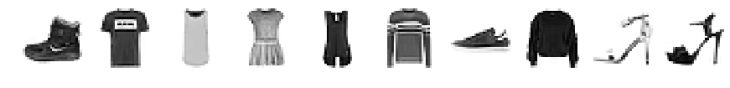
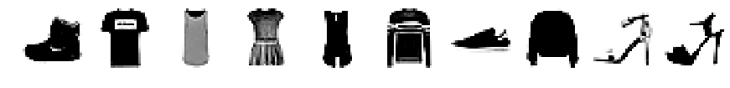
The more we train the autoencoder, the more accurate the coding and decoding will perform:
Original data:

Autoencoder’s output after:
- 100 epochs:

3-3) How to use the autoencoder as pre-trained model
To use this model as a pre-trained model we need to:
- load the model
- remove the decoder part (half of the encoder in general)
- freeze all the coder layers’ weights
- add layers (convolutional and/or fullyconnected)
Here is how to do each part:
pretrained_autoencoder = keras.models.load_model(MODEL_PATH + 'autoencoder.h5')
# display the summary to see the layers we need to remove
pretrained_autoencoder.summary()
Output:
Model: "model_1"
_________________________________________________________________
Layer (type)                 Output Shape              Param #
=================================================================
input_2 (InputLayer)         [(None, 28, 28, 1)]       0
_________________________________________________________________
conv2d_5 (Conv2D)            (None, 28, 28, 8)         80
_________________________________________________________________
max_pooling2d_2 (MaxPooling2 (None, 14, 14, 8)         0
_________________________________________________________________
conv2d_6 (Conv2D)            (None, 14, 14, 4)         292
_________________________________________________________________
max_pooling2d_3 (MaxPooling2 (None, 7, 7, 4)           0
_________________________________________________________________
conv2d_7 (Conv2D)            (None, 7, 7, 4)           148
_________________________________________________________________
up_sampling2d_2 (UpSampling2 (None, 14, 14, 4)         0
_________________________________________________________________
conv2d_8 (Conv2D)            (None, 14, 14, 8)         296
_________________________________________________________________
up_sampling2d_3 (UpSampling2 (None, 28, 28, 8)         0
_________________________________________________________________
conv2d_9 (Conv2D)            (None, 28, 28, 1)         73
=================================================================
Total params: 889
Trainable params: 889
Non-trainable params: 0
_________________________________________________________________
Adding layers and removing the decoder:
#removing decoder (last 4 layers)
x = pretrained_autoencoder.layers[-5].output
# Adding layers
x = Conv2D(32, (3, 3), activation='relu', padding='same')(x)
x = Conv2D(64, (3, 3), strides=2, activation='relu', padding='same')(x)
x = Conv2D(128, (3, 3), strides=2, activation='relu', padding='same')(x)
x = Flatten()(x)
x = Dense(128, activation='relu')(x)
# Adding a fully connected layer for the 10 classes 0 to 9
predictions = Dense(10, activation='softmax')(x)
model = Model(inputs=pretrained_autoencoder.input, outputs=predictions)
model.summary()
Output:

Model: "model_4"
_________________________________________________________________
Layer (type)                 Output Shape              Param #
=================================================================
input_2 (InputLayer)         [(None, 28, 28, 1)]       0
_________________________________________________________________
conv2d_5 (Conv2D)            (None, 28, 28, 8)         80
_________________________________________________________________
max_pooling2d_2 (MaxPooling2 (None, 14, 14, 8)         0
_________________________________________________________________
conv2d_6 (Conv2D)            (None, 14, 14, 4)         292
_________________________________________________________________
max_pooling2d_3 (MaxPooling2 (None, 7, 7, 4)           0
_________________________________________________________________
conv2d_7 (Conv2D)            (None, 7, 7, 4)           148
_________________________________________________________________
conv2d_20 (Conv2D)           (None, 7, 7, 32)          1184
_________________________________________________________________
conv2d_21 (Conv2D)           (None, 4, 4, 64)          18496
_________________________________________________________________
conv2d_22 (Conv2D)           (None, 2, 2, 128)         73856
_________________________________________________________________
flatten (Flatten)            (None, 512)               0
_________________________________________________________________
dense_4 (Dense)              (None, 128)               65664
_________________________________________________________________
dense_5 (Dense)              (None, 10)                1290
=================================================================
Total params: 161,010
Trainable params: 160,490
Non-trainable params: 520
_________________________________________________________________
We replaced the decoder by our own layers.
Freezing coder layers’ weights:
# freeze all layers of the pre-trained model
# we will only update the weights for the added layers
for layer in pretrained_autoencoder.layers:
    layer.trainable = False
Compile the model:
model.compile(optimizer='adam', loss='sparse_categorical_crossentropy', metrics=['sparse_categorical_accuracy'])
Here you can find my project:
https://github.com/Apiquet/transfer_learning_and_unsupervised_pre-training
Header image source: towardsdatascience

What’s Going down i am new to this, I stumbled upon this I’ve discovered
It absolutely useful and it has aided me out loads.
I’m hoping to give a contribution & assist other customers like its helped me.
Great job.
my homepage: What Is An Alpha Male
LikeLiked by 1 person
Thank you so much for sharing, it’s great to see that my work is helping other people!
LikeLike
Usually I do not read article on blogs, but I would like to say that this write-up very
forced me to check out and do it! Your writing style has been amazed me.
Thank you, quite nice post.
Stop by my blog post … w88
LikeLiked by 1 person
Thank you very much for your comment, I really appreciate it!
LikeLike
Great article, just what I wanted to find.
LikeLike
Glad to see that it was useful to you!
LikeLike
I am really impressed with your writing skills as
well as with the layout on your blog. Is this a paid theme or did
you modify it yourself? Anyway keep up the excellent quality writing,
it is rare to see a great blog like this one today.
LikeLiked by 1 person
Hello, thank you very much for your comment ! I only choose free themes that fit well with the content of my articles to avoid having to modify it. Spending less time designing the container allows me to spend more time on the content.
Its name is Gazette, described as a minimalist magazine-style theme 🙂
LikeLike