AI, Deep Learning, Python

Data Aug. and Generative auto-encoder

Python project, Tensorflow.

This article shows how to get familiar with Tensorflow and how to use its great tool TensorBoard.

We will train a CNN on the MNIST dataset with few samples and show how to artificially increase our dataset (rotation, zoom, contrast, etc) to improve its accuracy. Then, we will explain how to implement a generative autoencoder to “dream up” new digits to improve our accuracy on real digits.

GitHub link: https://github.com/Apiquet/Deep_learning_digit_recognition_and_creation

In this article, I will first give a quick summary of CNN, then show the capabilities of Tensorflow to build a CNN and how to monitor our results in TensorBoard. I will present how to display the results of different runs or models in the same graphs for comparison. Finally, I will show how to artificially augment our dataset (rotation, room, contrast).

I will finish with a generative auto-encoder to create new digit artificially!

Table of contents

1. Summary of CNN
2. Tensorflow: Convolutional layers available
3. TensorBoard
4. Increasing the dataset artificially
5. Better CNN to reach high accuracy
6. Generative autoencoder:

1 – Summary of CNN

Each neuron reacts to a patch of the previous layer, the further the layer is from the network input the more it has a generalized view on the image.
A convolutional layer consists of several successive layers called feature maps. All the “pixels” of a feature map have equal parameters contained in the associated kernel. Each layer therefore applies several filters to its inputs.

• Known architectures:
  • oNet-5 (1998): convolution and mean-pooling + tanh
  • AlexNet (2012): is similar to LeNet-5 but wider and deeper. First to not interpose pooling between each layer. Uses max-pooling. Reread. Dropped 50%. Artificially increased data: flipping and lighting changes. Uses LRN (Local Response Normalization) after some convolutional layers that lead the most activating neurons to inhibit neurons located at the same place in neighboring feature maps.
  • GoogLeNet: much deeper network. This is possible thanks to the presence of sub-networks called inception module which allows to use the parameters more efficiently. It has 10 times less parameters than AlexNet! ReLU used. 2 secondary classifiers were used in addition to the network.
  • ResNet: the much deeper winner: 152 layers. Possible thanks to skip connections: The signal supplied to one layer is also added to the output of a layer a little higher up in the stack. This is called residual learning. Instead of modeling a target function h (x), we model h (x) – x because we add the input x to the network output. Learning is accelerated because the network initially models the identity function. By adding many jump connections, we create a network that becomes a stack of residual units. Each residual unit consists of 2 convolution layers, batch normalization, ReLU activation, 3×3 kernels and no 1s.

Inception module:

• uses convolution of 1×1 in order to size shrink.
• Uses several convolutional layers in parallel which is equivalent to a very complex convolutive layer but with fewer parameters.
• The Inception module can be seen as a convolutive layer on vitamins.
• There are however more hyperparameters to adjust as there are for each convolutive layer in parallel.
• The module ends with a concatenation layer.

2- Tensorflow: Convolutional layer kinds

Good visualizations of the convolution process are available in this article.

To create convolutional layers, there are many options:

• conv1d(): used for inputs with 1 dimension (useful for NLP where a sentence can be represented as a table of word)
• conv3d(): for inputs with 3 dimensions (for instance in medical imaging)
• atrous_conv2d(): a convolutional layer with a dilatation operation. It inserts lines and columns of 0 (useful because we can have a larger receiver field without increasing calculation either parameters).
• conv2d_transpose(): over-samples an image. Inserts 0 between inputs. Useful for segmentation of images because with regular convolutional layers, the feature maps become smaller and smaller (if no padding used). We thus need a convolutional layer which over-samples to increase the output size.
• depthwise_conv2d(): applies each filter independently to each input dimension.
• separable_conv2d(): behaves as a depthwise_conv2d() but ends by applying a regular 1×1 convolutional layer to the feature maps.

a Conv2D implementation:

conv1 = tf.keras.layers.Conv2D(
    X_reshaped, filters=conv1_fmaps,
    kernel_size=conv1_ksize,
    strides=conv1_stride, padding="SAME",
    activation=tf.nn.relu, name="conv1")

The creation of complex neural networks for object detection, style transfer, segmentation, etc. are available in the next articles.

3 – TensorBoard

Thanks to the Tensorboard, we can visualize curves with scalars (accuracy, loss, etc.), histograms, graphs, etc.

First, I will explain how to visualize our neural network in the tensorboard. This allows us to keep a history of all the tested architectures. To be more precise, we can also add a “scope” to our code to give a name to each layer (or group of layers):

with tf.name_scope("output"):
   logits = tf.layers.dense(fc1, n_outputs, name="output")
   Y_proba = tf.nn.softmax(logits, name="Y_proba")

Thanks to this kind of implementation, the Tensorboard will organized our NN in a graph to simply visualize it:

We also have access to the history of each architecture to compare them.

Another feature is to visualize any scalar we want in different ways: graphs, histograms, etc. Thanks to it, we don’t need to manually save each scalar in a list, and then display graphs using matplotlib or any other similar library. Just add the scalars to the list of scalars to monitor, and Tensorflow will take care of the storage part to display beautiful graphs.

But that’s not all. We can also record the scalar for different NN architectures. Tensorboard will then display, with a different color, the evolution of a particular scalar for each architecture. We can easily compare them without having to save each log manually.

In the example below, I put a title in my log with the description of the NN architecture (2 convolutional layers, 3 convolutional layers, 3 convolutional layers with an artificially augmented dataset). I can now easily compare their performances.

...
accuracy_train_ = tf.summary.scalar('accuracy_train', accuracy_train)
... code ...

#merge all the scalars which need the same data
merged = tf.summary.merge([accuracy_train_, loss_, ...])

Then, in the epoch loop, we can evaluate the variables and write them to the Tensorboard:

summary_str = sess.run(merged, feed_dict={X: X_batch, y: y_batch})
# test accuracy needs X_test, y_test so we did not included it in "merged" which 
#needs X_train and y_train (in my code it's *_batch because I'm doing mini-batch GD)
test_summary_str = sess.run(accuracy_test_, feed_dict={X: X_test, y: y_test})
tf_tensorboard_writer.add_summary(summary_str, epoch) 
tf_tensorboard_writer.add_summary(test_summary_str, epoch)

We finally get this kind of representation in the Tensorboard:

4 – Increasing the dataset artificially

To increase the dataset we can rotate the images, apply a zoom, change the contrast, etc.

from scipy.ndimage import rotate
degrees = 10
samples_to_show = 5
for iteration in range(samples_to_show):
    plt.subplot(samples_to_show, degrees, iteration + 1)
    plot_image(rotate(X_reshaped[iteration], 20, reshape=False))

The code above allows to rotate 5 images. Other transformations are available on the GitHub project.

We can also change the contrast:

I created 1000 new images with a rotation of 10, 1000 with a rotation of -10, 1000 with a 0.8 zoom applied.

I first trained the model with 1000 handwritten numbers, I got an accuracy of 0.9188. Then I increased my dataset following the above plan. I got an accuracy of 0.9544 (accuracy tested on a separate test set). This is a good improvement!

5 – Better CNN to reach high accuracy

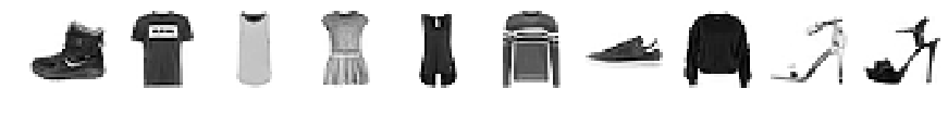
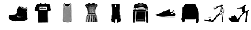
Thanks to data augmentation (rotation, zoom, contrast), we can get better results. I tried it on two different problems: the digit dataset and the fashion dataset of MNIST.

For both problem I got good results thanks to the following changes:

• not using pooling after each convolutional layer
• Batch normalization
• Data augmentation
• Dropout

I used 3 convolutional layers, 1 pooling and 2 fully-connected layers. I got 99.51% accuracy for the digit recognition task, 93.12% for the clothing classification with the fashion MNIST dataset. Both were achieved with the same neural network architecture. I could get better results with a deeper architecture but the main purpose here was to get familiar with the techniques above.

6 – Generative auto-encoder:

We often see advertisements from large companies like Google that have developed a neural network that can “dream”. They can “dream” by creating a new painting or a new sound that perfectly matches the style of a famous person (Picasso, Mozart, etc.). I wondered how these neural networks work and discovered the generative autoencoder.

I would like to thank Aurélien Geron once again for his amazing examples of neural networks.

For such a NN, we need to create an autoencoder. These works as follow:

It tries to represent the input with the neurons available in the Code section. Then it tries to reconstruct the input into output. We just want to create the Unit function where the output must be equal to the input! The difficulty here is to find an optimal representation of the input to correctly reconstruct the input. The less freedom there is in the code section, the more difficult the task.

With this architecture, we can do:

– Reduction of dimension

– Characteristic extraction

– Unsupervised pre-training

– Generative model

To build a deep autoencodeur, the autoencoders are stacked and each is driven in turn.

To regularize, one can either use dropout on its inputs or add a Gaussian noise on the input image but calculate the final error on the original image.

Dispersal is another type of constraint: add an appropriate term to the cost function to force the encoder to have for example only 5% of neuron in response very high at the same time (it forces it to extract that the most important). To know this term, one must first train the network without, then measure the average intensity of each neuron. If our objective is an average activation of 0.1 and a neuron at 0.3, we use the Kullback-Leibler divergence (which is the technique with the highest gradients (otherwise we would add the quadratic error: (0.3 – 0.1) ^ 2

There are also variational autoencoders:

• Probabilistic encoder (output partially defined by chance, even after the training, while the denoiser uses the chance that during the training)
• Generative autoencoder
• Comparable to RBM but easier to train and sampling is faster (with RBM it is necessary to wait for the network to stabilize in a “thermal equilibrium” before being able to sample another instance
• Produces a mean mu encoding and sigma standard deviation. It can then be used to generate new data after training by applying to the input of decoder, a code of average mu and standard deviation sigma.

There are also other types:

• contractor autoencoder to force similar images to have similar encoding
• GSN (generative stochastic network): denoiser capable of generating data
• WTA (winner-take-all): keeps only the neurons that are the most active to create hollow models
• GAN (generative adversarial network): a first network, the discriminant, is trained to differentiate true data from false. Meanwhile the generator learns to deceive the discriminant. But at the same time the discriminant learns to avoid the traps of the generator. It creates a very powerful generator, generating very realistic data.

Once the autoencoder is trained, we can apply a normal distribution to its decoder to create new samples!

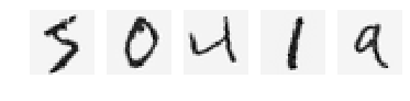
Here is what I got from an autoencoder with 1000 and 60,000 samples:

1000 samples in training:

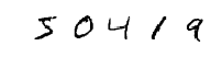
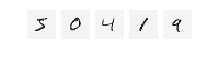
We can distinguish digits but it’s blurry. The following digits were created with a NN trained with 60,000 samples:

The following ones are 60 hand written digits:

The ones done by the autoencoder are a bit blurry but we can easily label them! With a bit of post processing on the digits, we could get a perfect result!

Here you can find my project:

https://github.com/Apiquet/Deep_learning_digit_recognition_and_creation