AI, Deep Learning, NN from scratch, Python

Neural network from scratch: Part 1; gradient descent

Python project.

This article explains the principle of gradient descent and its implementation :

1. Using the differential approach (2D example),
2. Using the perturbation approach (3D example),

GitHub link: https://github.com/Apiquet/neural_net_from_scratch

Table of contents

1. What is a Gradient Descent
   1. Differential approach with known functions
      • Code implementation in Python
      • How to avoid local minimum
      • Code implementation of momentum
   2. Perturbation approach with unknown functions
2. Conclusion

1- What is a Gradient Descent

Applied to a function, a gradient descent should find a path to a local minimum around the starting point. An example would be necessary to clarify its principle:

Above is a simple quadratic function. As shown on the figure, starting from the red point, the gradient descent should lead to the yellow one. It progresses step by step, down the slope.

The next chapters will clarify how gradient descent works to minimize functions through 2D and 3D examples. It will help to understand how it can make neural networks learn tasks. Because, finally, these networks are only high-dimensional functions.

1-1 Differential approach with known functions

The first approach that I will explain is used when the equation of the function is known. In this case, we can calculate its derivative. This derivative shows how to update the our position to minimize the function’s value.

For a quadratic function:  , the derivative is:

Below is a plot of these two functions:

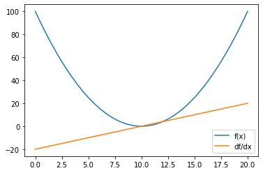
If we start a gradient descent from the point x=20, then f(20)=(20-10)^2=100. We can then use the derivative to know if we need to increase or decrease x to reach a lower point. The value of the derivative on x=20 is called the gradient and it goes to the opposite of the slop. Knowing this fact, we know that we need to update x on the opposite way.

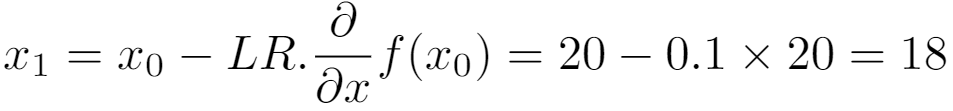
Evaluated on x=20, the derivative equals to 2.(20-10)=20 which is positive so we need to decrease x to reach a lower function’s value.

The last thing to set is the learning rate which is the size of the step we authorize the gradient descent to make. For instance, this value can be set to 0.1 but it depends of the application. The equation below shows the process to update x:

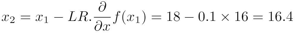
For the step 2, x has value 18 which is closer to the objective x=10, the global minimum of the function. We can then continue until we reach x=10:

The gradient descent should stabilize itself on the minimum. Close to x=10, for instance x=10.1 at the step n, we can calculate the value of the update:

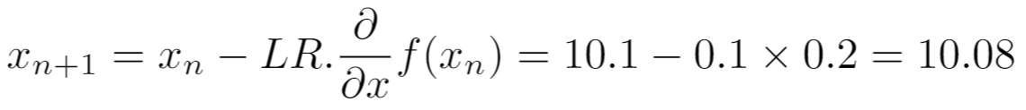
The update is only of 0.02. The closer we get from the minimum, the smaller are the updates.

1-1-a Code implementation in Python

The example above can be coded with few lines using numpy and sympy libraries. Matplotlib can also be used to plot graphs.

First we need to import these libraries:

import numpy as np
import matplotlib.pyplot as plt
from sympy import *

Then, we have to set the equation and calculate its derivative.

# create function
x = Symbol('x')
f = (x-10)**2

# calculate the derivative
df = f.diff(x)

# lambdify both functions
f = lambdify(x, f)
df = lambdify(x, df)

# evaluate
pts = np.linspace(0, 20)
plt.plot(pts, f(pts), label='f(x)')
plt.plot(pts, df(pts), label='df/dx')
plt.legend()
plt.show()

The code above plot the following graph:

Finally, the gradient descent can be programmed using the process explain above:

# maximum iteration to avoid calculating forever
max_iter = 300
# learning rate
lr = 0.05
# starting point
X0 = 30

# save iteration number to break if it reaches max_iter
cur_iter = 0
# saving each step to visualize it afterwards
steps = [X0]

# gradient descent
while True:
    # get closer to a local min
    X1 = X0 - lr * df(X0)
    # save step
    steps.append(X1)
    # calculate step size
    step_size = abs(X0 - X1)
    # save new step
    X0 = X1
    if cur_iter > max_iter:
        print("Max iter reached")
        break
    if step_size < 0.00001:
        print("Local min reached")
        break
    elif cur_iter%20 == 0:
        print("Iteration {} has x value {}".format(cur_iter, X1))
    cur_iter = cur_iter + 1    
print("The local minimum occurs at", X1)

The code above should return the following lines:

Iteration 0 has x value 28.0
Iteration 20 has x value 12.188379782630246
Iteration 40 has x value 10.266055892945824
Iteration 60 has x value 10.032346185398458
Iteration 80 has x value 10.003932541009512
Iteration 100 has x value 10.000478105179978
Local min reached
The local minimum occurs at 10.000088593855091

Finally, the visualization can be done using:

pts = np.linspace(-10, 30)
plt.plot(pts, f(pts), label='f(x)')
plt.plot(pts, df(pts), label='df/dx')
# change color to see GD progress
color = [item/255 for item in list(range(len(steps)))]
plt.scatter(steps, [f(x) for x in steps], label='Gradient descent', c=color)
plt.legend()
plt.show()

The graph shows how the gradient descent progressed step by step, down the slop.

1-1-b How to avoid local minimum

Unfortunately, functions can have many local minimums. The previous implementation stops the gradient descent at the first local minimum found. A technique to avoid that consists in adding a momentum to give speed to the descent. Thanks to it, the gradient descent can avoid some local minimum if they are not too deep.

The example bellow helps to understand the concept:

As shown above, momentum gives speed when descending the slope. It is obtained by considering the previous steps to make the next one. Older steps should be considered less than newer ones, so all previous steps should be multiplied by a factor between 0 and 1 (usually 0.9) at each step. In this case, the momentum at step n should be:

Thanks to the multiplication, only the recent steps done will be strongly considered.

1-1-c Code implementation of momentum

The implementation is very close to the one of the previous section. The only change is the addition of the momentum to every step. The code can be found at the following link.

1-2 Perturbation approach with unknown functions

The previous example is efficient when the function is know, but this is not always the case ! The perturbation approach can be used to minimize a function. This section will use a 3D example, the code above will show the function used:

import numpy as np
import matplotlib.pyplot as plt
from mpl_toolkits.mplot3d import Axes3D
from sympy import *

# function used
def f(x, y):
    return np.sin((x ** 2 + y ** 2))

x = np.linspace(-2, 2, 100)
y = np.linspace(-2, 2, 100)
X, Y = np.meshgrid(x, y)
Z = f(X, Y)

fig = plt.figure()
ax = plt.axes(projection='3d')
ax.contour3D(X, Y, Z, 50, cmap='winter')
ax.set_xlabel('x')
ax.set_ylabel('y')
ax.set_zlabel('z')
ax.view_init(60, 35)

The code above plots the function in 3D:

Of course, we will not use the equation to do the gradient descent in this section. We will start at (x,y) = (0,-1), and make a gradient descent capable of reaching the local minimum in 0, 0. Then, we will implement a momentum to avoid the local minimum in (0,0) to reach (0,2) which is the lowest point in the direction of the first slop starting at (0,-1).

Perturbation approach consists in using a little step dw to calculate the result of f(X0+dw,Y0)-f(X0,Y0). This calculation gives two crucial information :

• the sign indicates the direction : >0 means that dw step increased the result, so we need to go in the opposite way
• the value indicates how much dw step change the result, the higher the value, the steeper the slope.

Then we divide the result by the step done. This gives the gradient, and as in the previous section, it points to the opposite of the slop so we need to multiply it by -1.

Then, the next step can be calculated with the following equation which uses the learning rate (explained in the first section):

The following function calculates the gradient given the function, a point (x,y) and a step (default is 0.01):

def find_direction(X0, Y0, dw=0.01):
    X1 = X0 + dw
    Y1 = Y0 + dw
    grad_x = (f(X1,Y0)-f(X0,Y0))/dw
    grad_y = (f(X0,Y1)-f(X0,Y0))/dw
    return grad_x, grad_y

Then, the following code implements the gradient descent:

max_iter = 300
lr = 0.1
X0 = 0
Y0 = -1
cur_iter = 0
steps_x = [X0]
steps_y = [Y0]
steps_z = [f(X0, Y0)]

while True:
    # get closer to a local min
    grad_x, grad_y = find_direction(X0, Y0)
    X1 = X0 - lr*grad_x
    Y1 = Y0 - lr*grad_y
    # save step
    steps_x.append(X1)
    steps_y.append(Y1)
    steps_z.append(f(X1, Y1))
    # calculate step size
    step_size_x = abs(X0 - X1)
    step_size_y = abs(Y0 - Y1)
    # save new step
    X0 = X1
    Y0 = Y1
    if cur_iter > max_iter:
        print("Max iter reached")
        break
    if step_size_x < 0.00001 and step_size_y < 0.00001:
        print("Local min reached")
        break
    elif cur_iter%20 == 0:
        lr = lr*0.7
        print("Iteration {} has x value ({:.4f},{:.4f})".format(cur_iter,
                                                                X1, Y1))
    cur_iter = cur_iter + 1

The above code outputs:

Iteration 0 has x value (-0.0005,-0.8908)
Iteration 20 has x value (-0.0048,-0.0542)
Iteration 40 has x value (-0.0050,-0.0112)
Iteration 60 has x value (-0.0050,-0.0065)
Iteration 80 has x value (-0.0050,-0.0056)
Local min reached

and the result can be visualized:

fig = plt.figure(num=None, figsize=(8, 6), dpi=80, facecolor='w', edgecolor='k')
ax = plt.axes(projection='3d')
color = [item/255 for item in list(range(len(steps_x)))]
ax.scatter(steps_x, steps_y, steps_z, s=50, c=color)
ax.scatter(steps_x[0], steps_y[0], steps_z[0], s=100, c='red', label='Start GD')
ax.scatter(steps_x[-1], steps_y[-1], steps_z[-1], s=100, c='yellow', label='End GD')
ax.contour3D(X, Y, Z, 50, cmap='winter')
plt.title('Gradient descent without momentum stays in local minimum')
plt.legend()
ax.set_xlabel('x')
ax.set_ylabel('y')
ax.set_zlabel('z')
ax.view_init(65, 20)

To avoid the local minimum in (0,0), we can implement once again a momentum. This momentum can be achieved using the same method of considering the previous steps:

The code can be found here.

to get the following result:

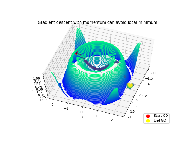
The gradient descent avoid the local minimum in (0,0) thanks to the speed given by the first slop. Then, the descent stops when reaching a flat place at (-0.25, 2). This is achieved by the formula of the gradient:

On a flat ground, f( Xo + dw, Yo) – f(Xo, Yo) is very small so the step update multiplied by the learning rate (~0.01) will be very small too.

Conclusion

In this article, we learned the principle of gradient descent in low dimensions and how to implement/visualize it. The next article will go deeper, we will learn how to implement a fully-connected neural network, which uses gradient descent.

Here you can find my project:

https://github.com/Apiquet/neural_net_from_scratch