

Neural Network from scratch: Part 3; Deep Learning Framework Implementation
Python project.
This article describes, step by step, how to implement a Deep Learning Framework from scratch using only the numpy library. It will show how to implement Convolution, Flatten, Max and Mean Pooling layers. It will also explain how to implement features such as: saving and loading a model to deploy it somewhere, getting its number of parameters, drawing learning curves, printing its description.
GitHub link: https://github.com/Apiquet/DeepLearningFrameworkFromScratch
Table of contents
- Summary of the previous article
- Convolution layer
- Principle
- Forward Pass Implementation
- Convolution on a 2D-image and 1 output feature map
- Convolution on a 1-channel images and multiple output feature maps
- Convolution on several multiple channels images and multiple output feature maps
- Backward Pass Implementation
- dx
- dw/db
- Flatten layer
- Multiple dimensions data to 1D predictions
- Implementation
- Max Pooling layer
- Principle of the max pooling
- Implementation
- Average pooling
- How to count the number of parameters of a neural network
- How to save and deploy homemade neural networks
- Example of use
1) Summary of the previous article
The previous article has already explained how to implement a fully-connected neural network from scratch using numpy. It has described the implementation of:
- activation functions (Sigmoid, ReLU, LeakyReLU
- Linear layer of neurons
- Softmax function
- Loss function (MSE: Mean Squared Error)
- Sequential module to create a neural network
- Training function (with one-hot encoding conversion, epoch and batch explanations)
If you need to read about any of these topics, please go to the article: https://apiquet.com/2020/05/02/neural-network-from-scratch-part-2/
It has also explained and illustrated the importance of having a source of non-linearity in a neural network.
This article will introduce and show the implementation of Convolution, Flatten, Max and Mean Pooling layers. It will also explain how to implement some good features provided by a Deep Learning Framework such as: saving and loading a model to deploy it somewhere, getting its number of parameters, drawing learning curves, printing its description and calculating confusion matrix.
2) Convolution layer
2-1) Principle
The previous article showed how to implement a succession of fully-connected layers. In these networks, each input is connected to a single neuron. The outputs of the neurons are connected to all the neurons of the next layer. The output values correspond to the outputs of the neurons of the last layer. However, this type of layer is not suitable for image processing: it is not at all invariant to translations or rotations and its size, in terms of number of neurons, increases very quickly with the number of inputs (for example 345600 for a picture of 720*480).
The convolutional layers are more adapted to image processing, they learn about image patches by following this equation:
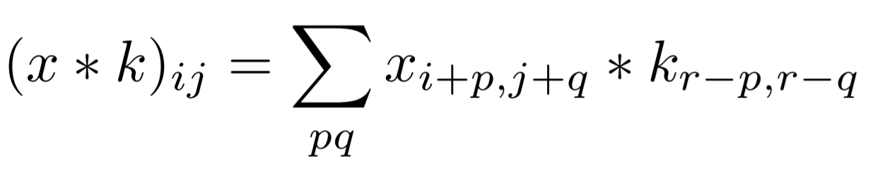
The principle of “kernel” is presented in the following figure.
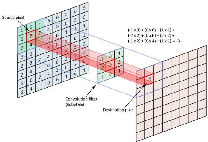
Each neuron of the convolution layer responds to the weighted sum of the neurons of the previous layer located in a geographical neighborhood. We then proceed in the same way for each neuron of each layer as shown in the next figure:
This describes the mechanism for calculating one channel of a convolution layer. However, they can have many other channels called feature maps. Each feature map is then calculated with its own kernel. This principal is very important because, once the feature map learned to respond to any pattern, this pattern can be anywhere in the image, we will catch it the same. This gives the translation equivariance to the convolution layer. Further in the article, we will see other mechanisms that produce local translation and rotation invariance.
2-2) Forward Pass Implementation
This layer is the hardest to implement but also the more interesting one. I have built it step by step:
- 1-channel input (2D data) and 1-channel output (1 feature map)
- several 1-channel images and several output’s feature maps
- several images of multiple channels and several output’s feature maps
2-2-a) Convolution on a 2D-image and 1 output feature map
First, we need to declare our input image and the one-channel kernel for a channel output:

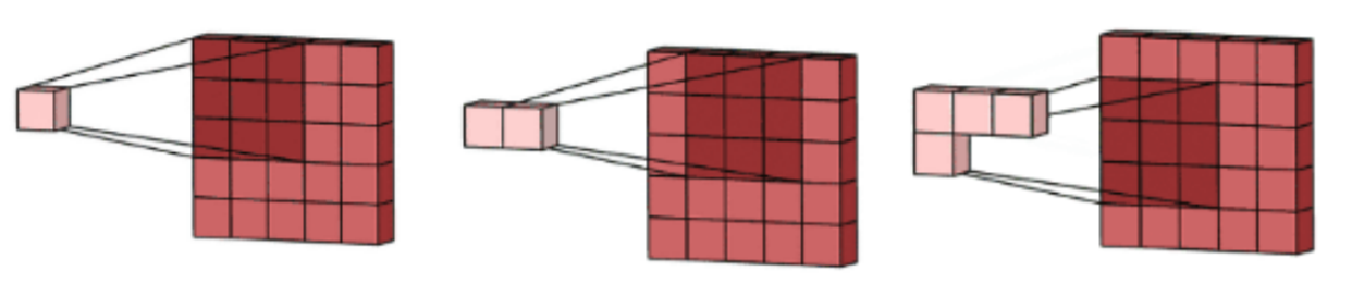
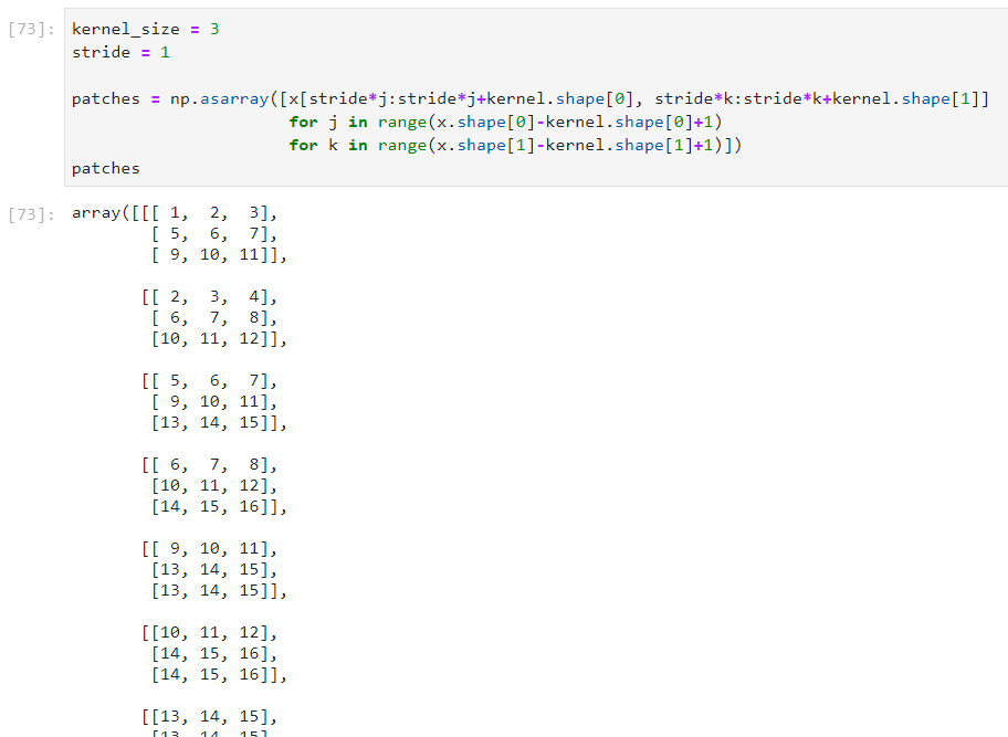
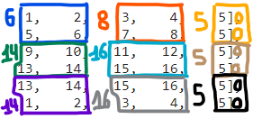
Then, a logic will be need to multiple, term by term, the kernel and the images patches (2D patches of kernel’s size (here 3×3). For that, we will first select the patches on the input images:
The patches should be selected as shown on the previous image until there is not more data (so 6 patches at all). Note: this technique use a stride of 1, which means that between two patches, we only move of one number to the left of to the bottom. We could also add a padding (0 values around the image) and we will see that for the backward pass.
Now, we need to multiple each patch by the kernel to achieve the convolution. For that, we will flat the patches and the kernel, then repeat the kernel n times to have two matrices of the same dimensions:
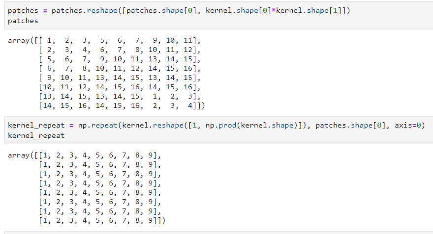
We can now easily multiply term by term and reshape the output data:
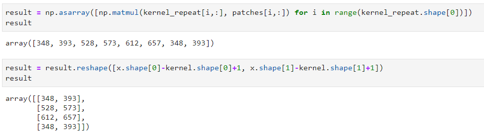
We finally got the convolution’s result between the input image and the kernel. This method is not optimal in term of calculation but this is the more understandable way I found.
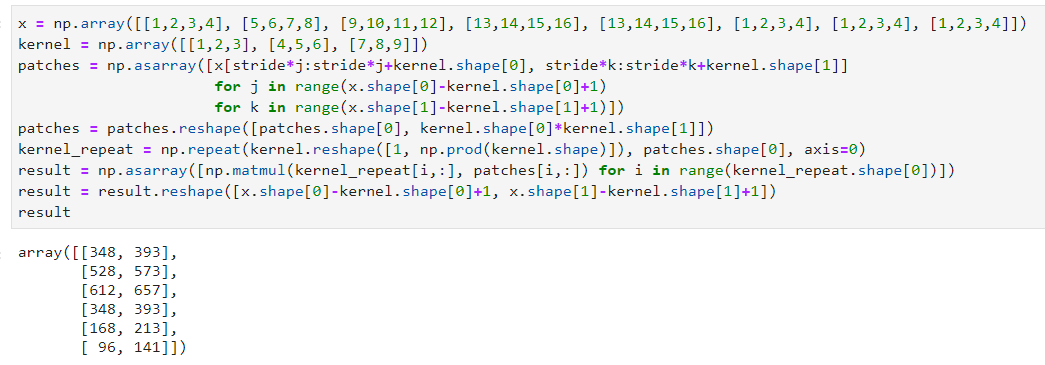
Here is the final code:
2-2-b) Convolution on a 1-channel images and multiple output feature maps
This section will be more complex because it introduces how to create multiple feature maps in the output data. This is achieved thanks to a multiple channels kernel.
First, we will create our input data and the kernel:
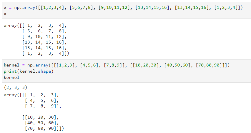
We now have 2-channels in our kernel. The next steps will be getting the patches from the input data, then flat the result. These two steps are equivalent to the ones done in the previous section as the input data did not change. However, the flat kernel will now have 2-channels:
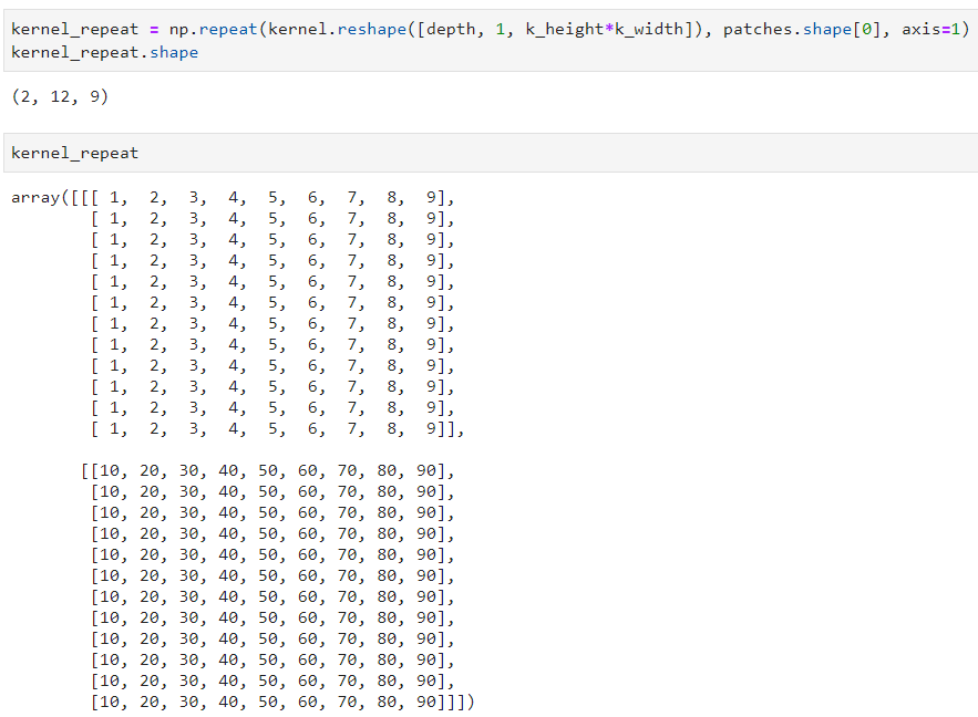
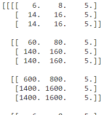
These 2-channels will produce 2-channels output data! We will repeat the calculation done on the previous section on the 2-channels:
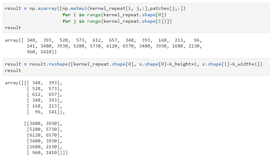
We now have the convolution’s results with 2 channels. These channels are called features maps.
2-2-c) Convolution on several multiple channels images and multiple output feature maps
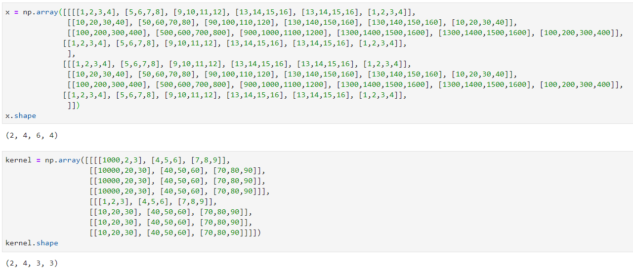
This section will achieve the final convolution function. It will process as input 4D data: multiple 3D data; NxCxWxH with N the number of samples, C the number of channels, W the width and H the height of the image or feature map. It will also create 4D outputs: multiple blocks of feature maps (NxFxWxH with F the number of feature maps). The created convolution will work with RGB images as input but also with feature maps input as the dimensions will be the same.
First, as usual, we will create the 4D input and now a 4D kernel: CxFxWxH with C the number of input channels, F the number of output features maps wanted, W the width and H the height.
Then we will adapt the calculations done on the previous section to the new channels (NxC for x and C for the kernel):
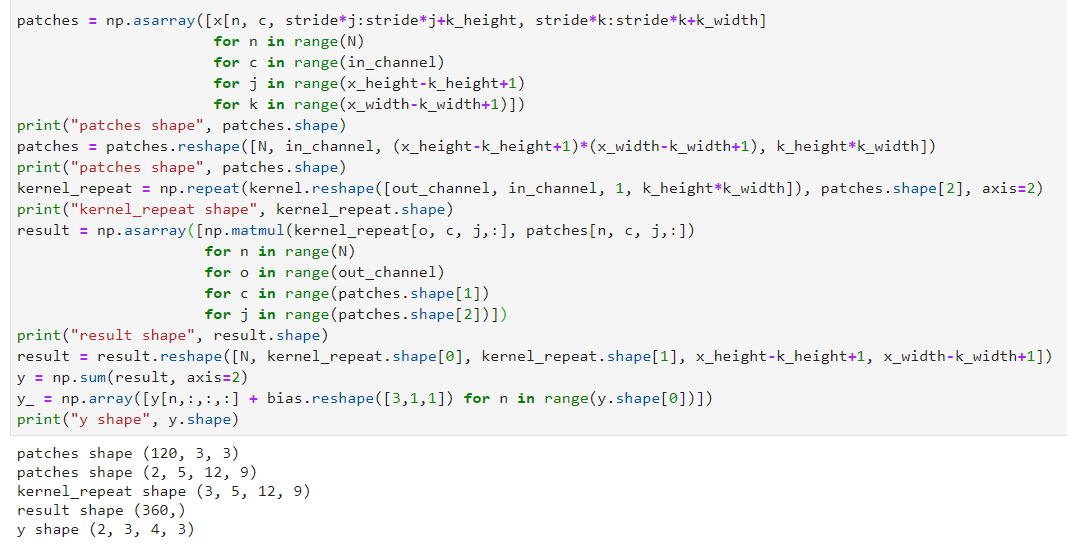
This produce the convolution result. However, something you may know is missing: the bias! Indeed, a bias should also be added to each feature map. This is simple to do, it will be a bias per feature map so only a vector of dimension F. Here is the final convolution function:
patches = np.asarray([x[n, c, stride*j:stride*j+k_height,
                        stride*k:stride*k+k_width]
                      for n in range(N)
                      for c in range(in_channel)
                      for j in range(x_height-k_height+1)
                      for k in range(x_width-k_width+1)])

patches = patches.reshape([N, in_channel,
                           (x_height-k_height+1)*(x_width-k_width+1),
                           k_height*k_width])

kernel_repeat = np.repeat(kernel.reshape([out_channel, in_channel, 1,
                                          k_height*k_width]),
                          patches.shape[2], axis=2)

result = np.asarray([np.matmul(kernel_repeat[o, c, j, :],
                               patches[n, c, j, :])
                     for n in range(N)
                     for o in range(out_channel)
                     for c in range(patches.shape[1])
                     for j in range(patches.shape[2])])

result = result.reshape([N, kernel_repeat.shape[0],
                         kernel_repeat.shape[1],
                         x_height-k_height+1, x_width-k_width+1])
y = np.sum(result, axis=2)
y = np.array([y[n,:,:,:] + self.bias for n in range(y.shape[0])])
The final code is available under the convolution class here: https://github.com/Apiquet/DeepLearningFrameworkFromScratch/blob/master/homemade_framework/framework.py
2-3) Backward Pass Implementation
2-3-1) dx
In the backward pass, we have to update the weight and bias of the convolution layer according to derivatives. This is achieved thanks to chain rules, already described in the previous article: https://apiquet.com/2020/05/02/neural-network-from-scratch-part-2/. In few words, the chain rule allows to find new values for each weight and bias to minimize the output error. We only need to derivate the weight and bias with respect to x. We also need to derivate x with respect to the weights to continue the back propagation through the previous layers.
These derivatives can also be written as convolutions, there are plenty of documentations online that found the demonstration if you are interested by it like me. The good point here is that we can use the convolution function previously created to both the forward and backward passes! All we have to do is transforming the kernel shape to do the derivative instead of the forward pass convolution:
k_reshaped = np.zeros_like(self.kernel)
for i in range(self.kernel.shape[-2]):
    for j in range(self.kernel.shape[-1]):
        k_reshaped[:, :, j, i] = np.flip(self.kernel[:, :, i, j])
This flip the kernel in a proper way to process the derivative according to demonstrations found online. Then we will need to reshape the data because, as you saw, the forward pass reduce the WxH dimension (if we do not add padding). For instance, with and image of 6×6 pixel, the convolution with a kernel of 3×3 will create an output of 4×4. So, at the backward pass, as the input comes from the end of the network, we will receive the 4×4 images and will need to produce a 6×6 output. This is achieved thanks to the padding, we will add 0 values around the 4×4 images to create a 8×8 images (so a border of 2 pixels of value 0). Then, the convolution between a 8×8 image and a kernel of 3×3 will create the good dimension of 6×6. This is important because the previous layer in the forward pass created a 6×6 output so, in the backward pass, this layer will need to receive a 6×6 input. This padding can be done as follow with numpy:
npad = ((0, 0), (0, 0), (self.k_height-1, self.k_height-1),
        (self.k_width-1, self.k_width-1))
dout = np.pad(dout, pad_width=npad, mode='constant', constant_values=0)
Then, we can do the convolution of the kernel and dout to obtain the derivative need to the next layer in the backward pass.
2-3-2) dw/db
We now need to update the weight and bias to reduce the output error. For that, we need to derivate the weight with respect to x, so we will process a convolution between dout (the input from the derivative of the previous layer) and x (the input of the forward pass). As the dimension won’t fit, we also need to process mean calculations:
N, F, W, H = dout.shape
mean_dout = np.mean(dout, axis=0, keepdims=True)
mean_x = np.mean(self.prev_x, axis=0, keepdims=True)
mean_x = np.repeat(mean_x, F, axis=1)

dk = self.convolution(mean_x, mean_dout)
dk = np.repeat(dk, self.kernel.shape[1], axis=1)
self.kernel = self.kernel - self.lr*dk
For the bias, this is much simpler, as this is only and addition to each feature map, there is not need to do convolution with x. We only need to do the mean of dout:
db = np.zeros_like(self.bias)
db = np.sum(dout, axis=(0, 2, 3))
self.bias = self.bias - self.lr*db.reshape(self.bias.shape)
This concludes the convolution class implementation. You can access the whole code on the link at the end of the article.
3) Flatten layer
3-1) Multiple dimensions data to 1D predictions
The purpose of flatten layers is to connect multi-dimensional data to 1D liner layer. They flat the whole matrix to achieve it.
3-2) Implementation
For the forward pass, we only need to flat the input numpy array and save the original shape to reconstruct it at the backward pass.
Forward pass: y = x.reshape([self.n, self.channel*self.width*self.height])
Backward pass: y = x.reshape([self.n, self.channel, self.height, self.width])
4) Max Pooling layer
4-1) Principle of the max pooling
To reduce the computing cost, neural networks implements pooling layers. This max pooling layer reduce generally by 4 the dimension by taking the maximum value of 2×2 patches. For instance, on an input of 14×14, the max pooling layer will produce an output of 7×7, its first element of coordinates (0,0) will be the max of the input coordinates: (0,0), (0,1), (1,0), (1,1).
4-2) Implementation
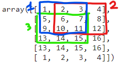
First, we need to create our input data:

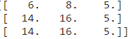
In this example, the max pooling should produce the following values for the first 2D block:
As you see, we need to add a padding (explained in the convolution implementation part) if the dimension is not a multiple of 2. This can be done with numpy:
npad = ((0, 0), (0, 0),
        (0, x_height % self.kernel_size),
        (0, x_width % self.kernel_size))
x = np.pad(x, pad_width=npad, mode='constant', constant_values=0)
This padding adds a column of 0 to the height and/or width if necessary. Then, we will need to find the maximum value of each 2×2 patches, but this won’t be enough. For the backward pass, we will need to reconstruct the forward pass input shape with the good values. To do so, we will need to save the shape of x, the indexes of the maximum values and their values:
self.x_max_idx = np.zeros(self.x_shape_origin)
y = np.zeros([x_n, x_depth,
              int(x_height/self.stride), int(x_width/self.stride)])

for n in range(x_n):
    for c in range(x_depth):
        for j in range(x_height//self.stride):
            for k in range(x_width//self.stride):
                i_max = np.argmax(
                    x[n, c,
                      self.stride*j:self.stride*j+self.kernel_size,
                      self.stride*k:self.stride*k+self.kernel_size])
                idx = [int(i_max > 1) + self.stride*j,
                       int(i_max == 1 or i_max == 3) + self.stride*k]
                self.x_max_idx[n, c, idx[0], idx[1]] = 1
                y[n, c, j, k] = x[n, c, idx[0], idx[1]]
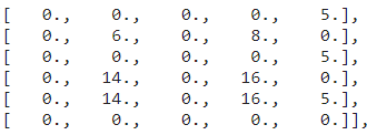
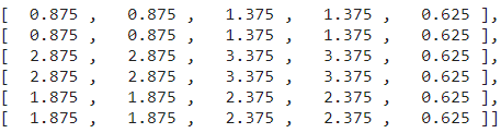
This create the output value as follow:
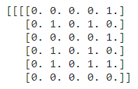
You can see that the first 2D block corresponds to the example given above. We also created the object x_max_idx to save the indexes of each maximum value. This is essential for the backward pass because we will receive as input data these block of 3×3 values and will need to produce the forward pass input shape: 5×6. So we will create a new numpy array of the good shape and then, we will map the 3×3 values to the good indexes in the 5×6 data.
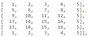
As it is easier through an example, we will take the same one. This max pooling:
will create this max_x_idx object:
This array as 1 values where we found the max values. Now, for the backward propagation, we will need to remap the input of 3×3 to these coordinates. For instance, if the backward pass receive as input:
We will need to create this array:
to pass it to the next layer. This is achieved by the following code:
dy = np.zeros(self.x_shape_origin)
x_n = self.x_shape_origin[0]
x_depth = self.x_shape_origin[1]
x_height = self.x_shape_origin[2]
x_width = self.x_shape_origin[3]

for n in range(x_n):
    for c in range(x_depth):
        for j in range(int(x_height)):
            for k in range(int(x_width)):
                dy[n, c, j, k] = self.x_max_idx[n, c, j, k] *\
                dout[n, c, j//self.stride, k//self.stride]
5) Average pooling
Max and Average pooling follow the same principle, but instead of taking the max value, the average pooling do a mean calculation. The code will be simpler because we do not need anymore to get indexes of values taken. For the forward pass, we only need to process the mean calculation on 2×2 patches:
for n in range(x_n):
    for c in range(x_depth):
        for j in range(x_height//self.stride):
            for k in range(x_width//self.stride):
                y[n, c, j, k] = np.mean(
                    x[n, c,
                      self.stride*j:self.stride*j+self.kernel_size,
                      self.stride*k:self.stride*k+self.kernel_size])
And finally, for the backward pass, as each value count in the output with a 1/4 factor, we juste need to remap each value to the good patches and divide it by 4. In the previous example, this input:
The forward pass will produce:
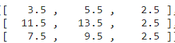
and if we send this matrix to the backward pass, it will produce:
With the following code:
for n in range(x_n):
    for c in range(x_depth):
        for j in range(int(x_height)):
            for k in range(int(x_width)):
                dy[n, c, j, k] = dout[n, c, j//self.stride,
                                      k//self.stride] / 4
6) How to count the number of parameters of a neural network
In a Deep Learning framework, we need some useful methods such as getting the number of parameters. For that, a user should only call model.getParametersCount(). As described in the previous article, our model is a Sequential model composed of each layer chosen by the user. This model calls every layer in sequence for the forward pass and reverses the order for the backward pass. We can also create other functions such as getParametersCount() which calls every layer to get their parameters count.
In the sequential class, we will add the function that get the parameters count of every layer:
def getParametersCount(self):
    parametersCount = 0
    for layer in self.model:
        parametersCount = parametersCount + layer.getParametersCount()
    return parametersCount
We will also add in the mother class a function getParametersCount() which returns 0 by default. We will then only need to overwrite this function in the child classes that has parameters. For instance the linear or convolution classes:
def getParametersCount(self):
    return np.prod(self.weight.shape) + np.prod(self.bias.shape)
We finally only need to call model.getParametersCount() to get the number of parameters of our neural network. This is useful to compare the complexity of models.
7) How to save and deploy homemade neural networks
Creating a method for saving and loading a model will follow the same example seen in the previous section. We will add a main method in the sequential class, then we will add a function in the layers with parameters to save. This method will be very useful because it allows to train a model on a computer and save it. You can then deploy it on a RaspBerry Pi or anywhere else and only load the weights saved to get the same accuracy for your task.
These methods will be simply called model.save(path) and model.load(path), here is the implementation in the sequential class:
def save(self, path):
    for i, obj in enumerate(self.model):
        params = obj.save(path, str(i))

def load(self, path):
    for i, obj in enumerate(self.model):
        params = obj.load(path, str(i))
As you can notice, we need to give a path to know where to save the weights. However, we need to find a way to load the good weights to the good layers. For that, I have chosen to give the layer number to save it in the file name. Finally, in the layers with weights to save, we only need to implement this method with numpy method .tofile(f) and np.fromfile(f). Here is an example for the convolution layer:
def save(self, path, i):
    with open(path + self.type + i + '-weights.bin', "wb") as f:
        self.kernel.tofile(f)
    with open(path + self.type + i + '-bias.bin', "wb") as f:
        self.bias.tofile(f)

def load(self, path, i):
    with open(path + self.type + i + '-weights.bin', "rb") as f:
        self.kernel = np.fromfile(f).reshape([self.out_channels,
                                              self.in_channels,
                                              self.k_height,
                                              self.k_width])
    with open(path + self.type + i + '-bias.bin', "rb") as f:
        self.bias = np.fromfile(f).reshape([self.out_channels, 1, 1])
We also implement an empty function save(i, path), load(i, path) in the mother class.
These function will create the following files:
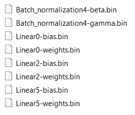
We can then use it as follow:
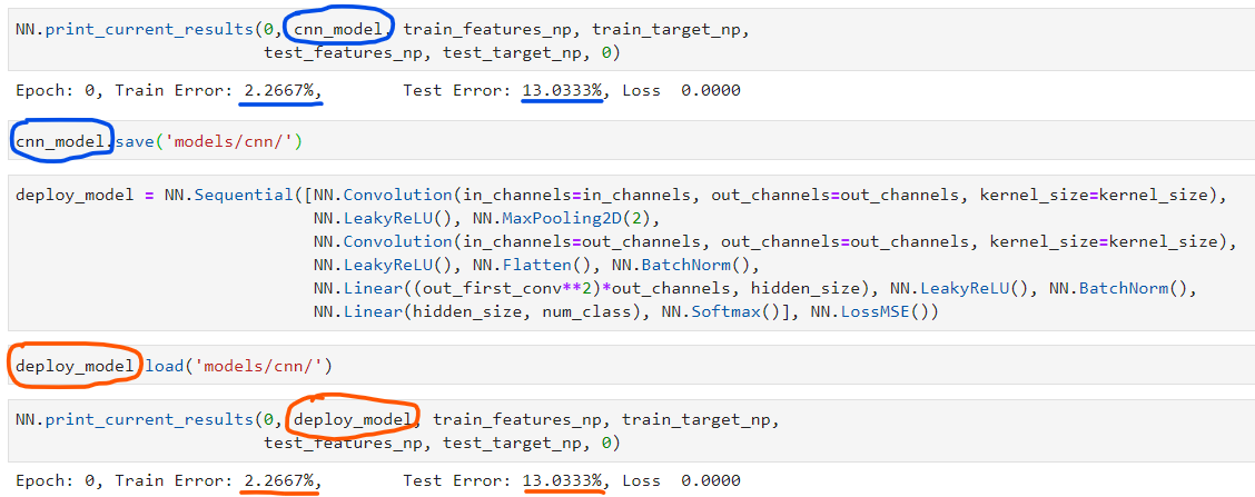
We can only create a python script on a deployed machine with a line for the model declaration and a line to load the weights of a model previously trained. Our model is then ready for inferences.
8) Example of use
You have a complete example of use of the Deep Learning framework on the following notebook: https://github.com/Apiquet/DeepLearningFrameworkFromScratch/blob/master/cnn_example.ipynb
Here is the example of implementation:
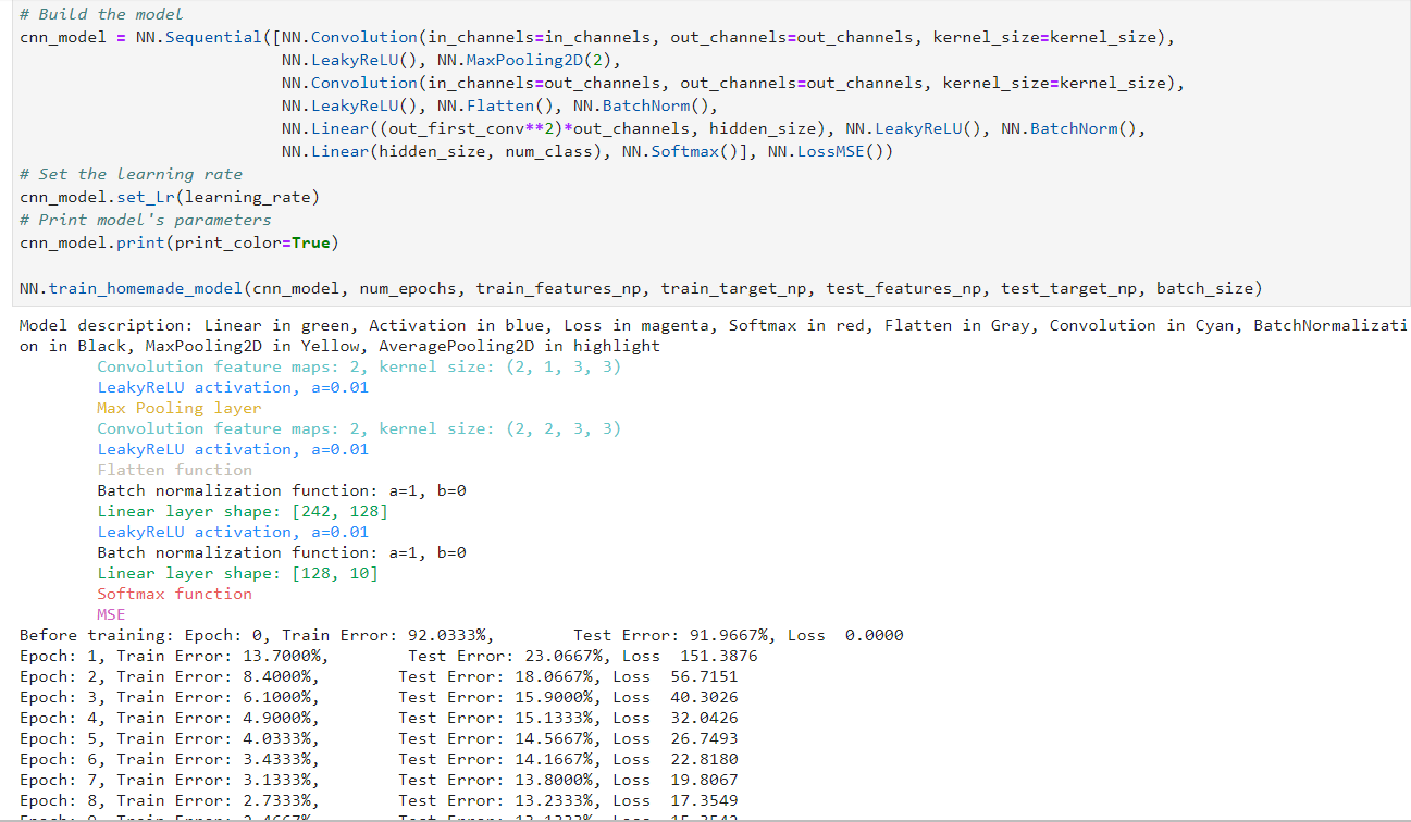
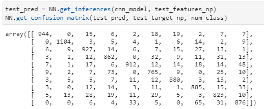
Some other methods are implemented in the framework but not described in this article such as model.set_lr(learning_rate) and model.print() which displays the model description in color if we want. We can also print the confusion matrix and the learning curves to analyze the results:
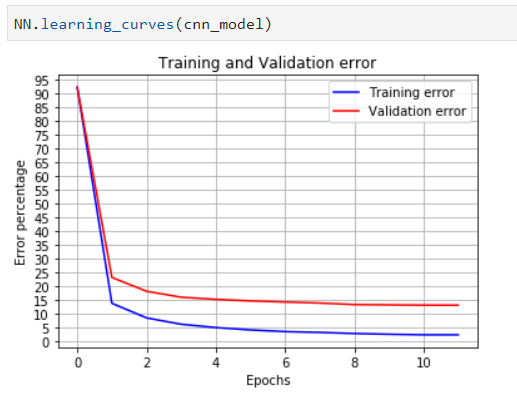
These curves are important to analyze the neural network learning to detect problems such as overfitting explained in previous articles.
Here you can find my project:
https://github.com/Apiquet/DeepLearningFrameworkFromScratch
Image header from: medium.com
