

SSD300 implementation
Python project, TensorFlow.
This article describes how to implement a Deep Learning algorithm for object detection, following the Single Shot Detector architecture. It explains the implementation of the VGG16 backbone network, the SSD cone, the default box principle and the convolutions used to predict the box classes and to regress the offsets for their location. Finally, how to convert the .xml annotations to data used by such a network for training.
GitHub link: https://github.com/Apiquet/Tracking_SSD_ReID
First, I will share the notes I have taken from the original paper: https://arxiv.org/pdf/1512.02325.pdf. Then, I will describe how I have implemented the VGG16 architecture, base network of the SSD, and the entire SSD architecture. The last sections will be dedicated to the database management (Pascal VOC 2012) and the neural network’s training.
Table of contents
- Paper
- Overview
- Principal
- The model
- Training
- VGG16
- SSD implementation
- Backbone
- Cone
- Confidence and loc
- Convolutions
- Default boxes
- Non-max suppression
- Losses
- Database management
- Read and parse annotations
- Create the ground truth from annotations
- Unoptimized version
- Optimized version
- confs_gt and locs_gt verification
- IoU and default boxes verification
- Offsets verification
- ground truth confs and locs verification
- Training
- Load pre-trained weights
- Optimizer and gradient calculation from loss
- Training function
- Get model’s results
- Draw predictions and ground truth on images
- Draw predictions on video
- Conclusion
1) Paper
1-1) Overview
- Deep neural network used for object detection
- Default set of bounding boxes of different aspect ratios and scales (per feature map)
- At prediction time: scores for the presence of each object class in each default box
- also produces adjustments to the box to better match object shape (offsets from the default box to the ground truth)
- Two possible input resolution : 300×300, 512×512
- High speed network mainly due to the elimination of bounding box proposals and resampling stage
- Small convolutional filters are used to predict object categories and offsets in bounding box locations
- Detection at different scales is allowed by using these filters on different feature maps
1-2) Principal
- At training time, SSD needs input images and ground truth boxes (for each object to detect)
- For each default box at each scale, offsets (to the ground truth box) and confidence for all object categories are predicted
- Default boxes are selected as positives and the rest as negatives: if there are close to the ground truth (several boxes can be matched for one ground truth box)
- The loss is a weighted sum between localization loss (smooth L1) and confidence loss (softmax loss: softmax activation + cross entropy loss)
1-3) The model
- Produces fixed-size collection of bounding boxes and scores for the presence of object class instances
- Non-maximum suppression is added to produce final detection
- VGG-16 is used as base network for high quality image classification
- Auxiliary structure is then added to produce detections with:
- Multi-scale feature maps: layers that decrease in size progressively (for multi-scale detection)
- Convolutional predictor: each feature map can produce a fixed set of detection using a set of convolutional filters. For a feature layer of nxm with p channels, the basic element for predicting parameters of a detection is 3x3xp small kernel that produce a score for a category, or a shape of offset relative to the default box. At each of the mxn location where the kernel is applied, it produces an output value
- Default boxes: the set of default bounding boxes is fixed in position. At each feature map, offsets are calculated relative to the default box shapes. So, as we have 4 offsets (center cx, cy and with/height) and a confidence for c classes, it leads to (c+4)*kmn outputs for mxn feature map with k the number of ground truth.
1-4) Training
- ground truth information needs to be assigned to specific outputs in the fixed set of detector outputs
- Once the assignment is determined, the loss function and back propagation are applied end-to-end
- Also need to choose the set of default boxes and scales for detection
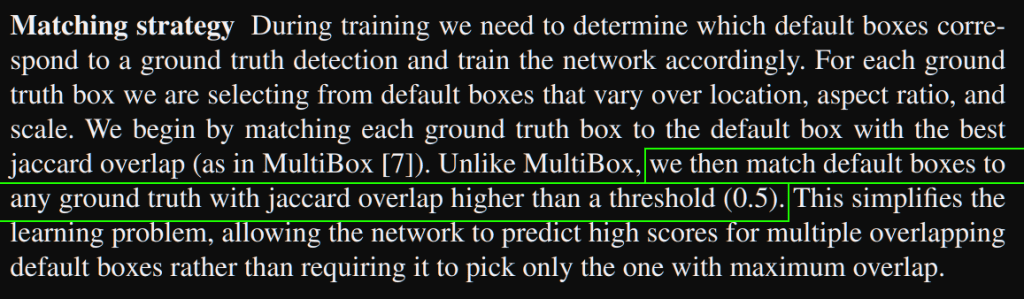
- Matching strategy: must determine which default boxes correspond to the ground truth one. This selection starts with the best jaccard overlap, then all boxes with a jaccard overlap > 0.5. This simplifies the learning problem, allowing the network to predict high scores for multiple overlapping default boxes rather than requiring picking only the one with maximum overlap.
- The loss is the weighted sum of localization loss and confidence loss with N the number of matched default boxes:

- If N=0, Lglobal = 0
- Lloc is a smooth L1 between predicted box and the ground truth (for center cx,cy and width/height)
- Lconf is a softmax loss (softmax activation + cross entropy loss: sum of negative logarithm of the probabilities)
- a was set to 1 (found with cross validation)
- possible aspect ratios: 1, 2, 3, 1/2, 1/3
- min size of default box over the network: 0.2, max: 0.9
- width = size * sqrt(ratio), height = size / sqrt(ratio)
- each default box has location: ((i+0.5)/|fk|, (j+0.5)/|fk|) with |fk| the size of the k-th square feature map (i and k are in [0, |fk|)
- Hard negative mining: after matching step most of the boxes are negatives, this leads to significant imbalance between positive and negative training examples. Instead of using all negative examples, they are sorted using the highest confidence loss for each default box and pick the top ones so that the ratio neg/pos is at most 3:1 (produce faster optimization and more stable training)
- Data augmentation: each image is randomly sampled by one of the following options:
- use initial image
- sample a patch so that the minimum jaccard overlap with objects is 0.1, 0.3, 0.5, 0.7 or 0.9
- Randomly sample a patch
- The size of sampled patch is in [0.1, 1] of the original image size, aspect ratio is between 1/2 and 2. The patch is kept if the center of the ground truth is in it
- Each sampled patch is resized to fixed size and horizontally flipped with probability=0.5
- Other photo-metric distortions are applied
2) VGG16
VGG16 has the following architecture:
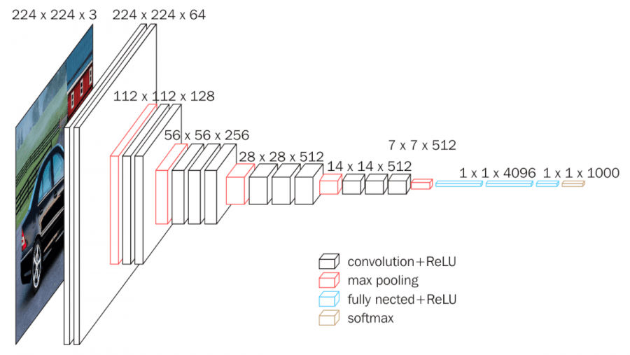
Each white block is a convolution with its dimensions (width, height, depth). The depth corresponds to the features maps. I have describes the convolution layers (principal, forward and backward passes implementation) in the following article at section 2: https://apiquet.com/2020/07/18/deep-learning-framework-from-scratch-part-3/.
Contrary to the next mentioned article, where I explained the convolution layer implementation with NumPy, we will use here TensorFlow. This library will help saving time because a line of code will be enough:
convolution_layer = Conv2D(input_shape=input_shape, filters=64,
                           kernel_size=(3, 3), padding="same",
                           activation="relu", name="convolution1")
The filters argument refers to the number of feature maps, padding “same” add padding to the input image to get the same resolution in output. For more details about the parameters’ purpose: https://apiquet.com/2020/07/18/deep-learning-framework-from-scratch-part-3/ (I explain there the purpose and implementation (with NumPy) of convolution layers, padding and activation functions like ReLU).
We can now declare all the layers:
self.conv_1_1_64 = Conv2D(input_shape=input_shape, filters=64, kernel_size=(3, 3),
                          padding="same", activation="relu", name="Conv1_1")
self.conv_1_2_64 = Conv2D(filters=64, kernel_size=(3, 3), padding="same", activation="relu", name="Conv1_2")
self.maxpool_1_3_2x2 = MaxPool2D(pool_size=(2, 2), strides=(2, 2), padding='same')

self.conv_2_1_128 = Conv2D(filters=128, kernel_size=(3, 3), padding="same", activation="relu", name="Conv2_1")
self.conv_2_2_128 = Conv2D(filters=128, kernel_size=(3, 3), padding="same", activation="relu", name="Conv2_2")
self.maxpool_2_3_2x2 = MaxPool2D(pool_size=(2, 2), strides=(2, 2), padding='same')

self.conv_3_1_256 = Conv2D(filters=256, kernel_size=(3, 3), padding="same", activation="relu", name="Conv3_1")
self.conv_3_2_256 = Conv2D(filters=256, kernel_size=(3, 3), padding="same", activation="relu", name="Conv3_2")
self.conv_3_3_256 = Conv2D(filters=256, kernel_size=(3, 3), padding="same", activation="relu",  name="Conv3_3")
self.maxpool_3_4_2x2 = MaxPool2D(pool_size=(2, 2), strides=(2, 2), padding='same')

self.conv_4_1_512 = Conv2D(filters=512, kernel_size=(3, 3), padding="same", activation="relu", name="Conv4_1")
self.conv_4_2_512 = Conv2D(filters=512, kernel_size=(3, 3), padding="same", activation="relu", name="Conv4_2")
self.conv_4_3_512 = Conv2D(filters=512, kernel_size=(3, 3), padding="same", activation="relu", name="Conv4_3")
self.maxpool_4_4_2x2 = MaxPool2D(pool_size=(2, 2), strides=(2, 2), padding='same')
self.conv_5_1_512 = Conv2D(filters=512, kernel_size=(3, 3), padding="same", activation="relu", name="Conv5_1")

self.conv_5_2_512 = Conv2D(filters=512, kernel_size=(3, 3), padding="same", activation="relu", name="Conv5_2")
self.conv_5_3_512 = Conv2D(filters=512, kernel_size=(3, 3), padding="same", activation="relu", name="Conv5_3")
self.maxpool_5_4_2x2 = MaxPool2D(pool_size=(2, 2), strides=(2, 2), padding='same')

self.flatten_6_1 = Flatten()
self.dense_6_2_4096 = Dense(4096, activation='relu')
self.dense_6_3_4096 = Dense(4096, activation='relu')
self.dense_6_4_10 = Dense(10, activation='softmax')
We can then create our model with all these layers:
self.model = keras.models.Sequential([
             self.conv_1_1_64,
             self.conv_1_2_64,
             self.maxpool_1_3_2x2,
             # Stage 2
             self.conv_2_1_128,
             self.conv_2_2_128,
             self.maxpool_2_3_2x2,
             # Stage 3
             self.conv_3_1_256,
             self.conv_3_2_256,
             self.conv_3_3_256,
             self.maxpool_3_4_2x2,
             # Stage 4
             self.conv_4_1_512,
             self.conv_4_2_512,
             self.conv_4_3_512,
             self.maxpool_4_4_2x2,
             # Stage 5
             self.conv_5_1_512,
             self.conv_5_2_512,
             self.conv_5_3_512,
             self.maxpool_5_4_2x2,
             # Stage 6
             self.flatten_6_1,
             self.dense_6_2_4096,
             self.dense_6_3_4096,
             self.dense_6_4_10
         ])
This model’s implementation can be moved to a class:
from tensorflow import keras
from tensorflow.keras.layers import Conv2D, MaxPool2D, Dense, Flatten
class VGG16():
    def __init__(self, input_shape=(224, 224, 3)):
        super(VGG16, self).__init__()
            ''' Available layers
                Typo: layerType_Stage_NumberInStage_Info '''
            self.conv_1_1_64 = Conv2D([...])
            [...]
            self.dense_6_4_10 = Dense(10, activation='softmax')

    def getModel(self):
        return keras.models.Sequential([...])
Then we can import the class and then get the model summary:
from models.VGG16 import VGG16
import tensorflow as tf
keras = tf.keras

VGG16_model = VGG16().getModel()
VGG16_model.compile(optimizer=keras.optimizers.Adam(lr=0.001),
                    loss=keras.losses.categorical_crossentropy,
                    metrics=['accuracy'])
VGG16_model.summary()
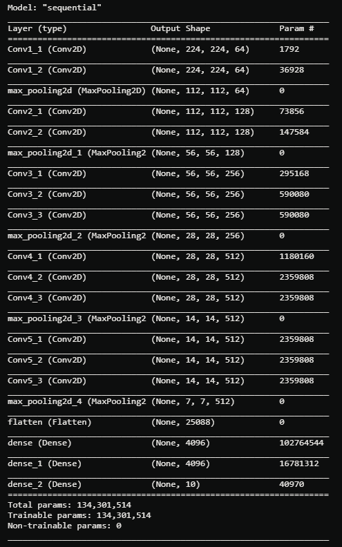
This summary allows to verify the resolution of each convolution.
3) SSD implementation
This part will be divided into several sections illustrated here:
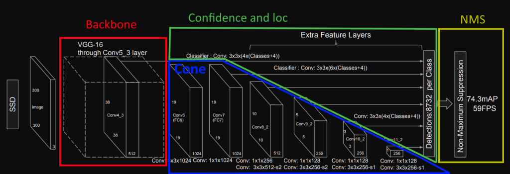
3-1) Backbone
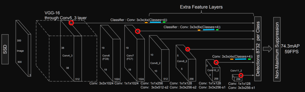
First, we need to look at how SSD architecture uses the VGG16 one:
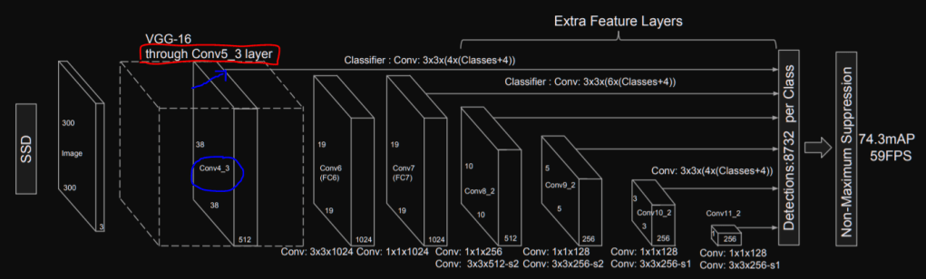
We can notice that SSD uses the VGG16 architecture until the conv5_3 layer (red rectangle) and it also uses the output of the conv4_3 layer to predict boxes in the image. We can then add two methods to our VGG16 class:
- a method that returns the VGG16 architecture until the conv4_3
- a method that returns the rest of the layers until conv5_3
def getUntilStage4(self):
         return keras.models.Sequential([
             self.conv_1_1_64,
             self.conv_1_2_64,
             self.maxpool_1_3_2x2,
             # Stage 2
             self.conv_2_1_128,
             self.conv_2_2_128,
             self.maxpool_2_3_2x2,
             # Stage 3
             self.conv_3_1_256,
             self.conv_3_2_256,
             self.conv_3_3_256,
             self.maxpool_3_4_2x2,
             # Stage 4
             self.conv_4_1_512,
             self.conv_4_2_512,
             self.conv_4_3_512])

def getStage5(self):
         return keras.models.Sequential([
             self.maxpool_4_4_2x2,
             self.conv_5_1_512,
             self.conv_5_2_512,
             self.conv_5_3_512])
Thanks to these methods, we know have the backbone implemented.
3-2) Cone
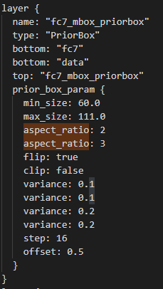
As we have the resolutions of the convolutions displayed in the SSD illustration and the code available, this will not be hard to implement it. The resolutions in the illustration will allow us to verify our implementation and we can use the official code to find each convolution’s parameters. As the official code uses Caffe, we have access to the convolutions’ implementation in the prototxt. For instance, we can see how the authors converted the fc6 layer to a convolution:

We can see the layer name and type in blue and its parameters in red, and its activation function ReLU. This gives us all the necessary information:
self.stage_6_1_1024 = Conv2D(filters=1024,
                             kernel_size=(3, 3),
                             adding="same",
                             activation="relu",
                             dilation_rate=6,
                             name="FC6_to_Conv6")
We can then do the same for all the layers, then, create a method ca implements the cone. This method will allow us to verify the resolution of each convolution. The following function should be created in the SSD300 class (with all the layers implemented like self.stage_6_1_1024 shown previously):
def getCone(self):
         return keras.models.Sequential([
             self.VGG16_stage_4,
             self.VGG16_stage_5,
             self.stage_6_1_1024,
             self.stage_7_1_1024,
             self.stage_8_1_256,
             self.stage_8_2_512,
             self.stage_9_1_128,
             self.stage_9_2_256,
             self.stage_10_1_128,
             self.stage_10_2_256,
             self.stage_11_1_128,
             self.stage_11_2_256])
Then we can call this method and run the .summary() function to get the resolution of each convolution:
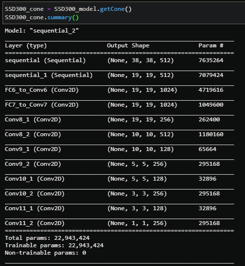
The first two sequential layers are stage 4 and 5 from VGG16 that we verified in the previous section. The next layers are the “cone” layers, each resolution corresponds to the one illustrated in the paper so we can go to the next step.
3-3) Confidence and loc
3-3-a) Convolutions
Please refer to the 1-c and 1-d sections to have more information about confidence and localization regression. I will only give a summary here:
- Default boxes are implemented, the model must find the good one for each object and its offsets (cx, cy, width, height) to adapt it to perfectly fit the object
- These default boxes are implemented on several stages in the cone to have a multi-scale detection
We have multiple information in the SSD’s representation that we can mark as follows:
This illustration gives us the following information:
- red: the stage to attach convolutions dedicated to confidence and localization regression
- orange: the number of default boxes per localization for the stage
- blue: parameter for the convolution dedicated to the confidence (for each box we have num_classes possibilities)
- green: parameter for the convolution dedicated to the localization (for each box we have 4 different offsets: cx, cy, width, height)
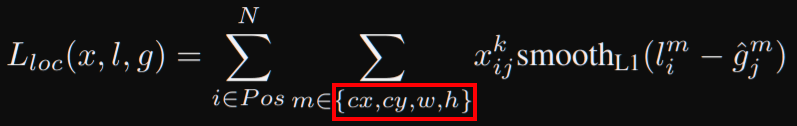
The paper confirms the offsets to regress in section 2.2:

We can also see it in the localization loss equation:
The number of default boxes is described in section 3.1:

This confirms that we need 4 default boxes for the stages 4, 10 and 11. 6 default boxes are implemented for the other stages (7, 8 and 9). There is also valuable information about normalization for the one of the stage 4. The following code implements the layers needed:
''' Confidence layers for each block '''
self.stage_4_batch_norm = tf.keras.layers.BatchNormalization()
self.stage_4_conf = Conv2D(filters=4*num_categories, kernel_size=(3, 3), padding="same", name="conf_stage4")
self.stage_7_conf = Conv2D(filters=6*num_categories, kernel_size=(3, 3), padding="same", name="conf_stage7")
self.stage_8_conf = Conv2D(filters=6*num_categories, kernel_size=(3, 3), padding="same", name="conf_stage8")
self.stage_9_conf = Conv2D(filters=6*num_categories, kernel_size=(3, 3), padding="same", name="conf_stage9")
self.stage_10_conf = Conv2D(filters=4*num_categories, kernel_size=(3, 3), padding="same", name="conf_stage10")
self.stage_11_conf = Conv2D(filters=4*num_categories, kernel_size=(3, 3), padding="same", name="conf_stage11")

''' Localization layers for each block '''
self.stage_4_loc = Conv2D(filters=4*4, kernel_size=(3, 3), padding="same", name="loc_stage4")
self.stage_7_loc = Conv2D(filters=6*4, kernel_size=(3, 3), padding="same", name="loc_stage7")
self.stage_8_loc = Conv2D(filters=6*4, kernel_size=(3, 3), padding="same", name="loc_stage8")
self.stage_9_loc = Conv2D(filters=6*4, kernel_size=(3, 3), padding="same", name="loc_stage9")
self.stage_10_loc = Conv2D(filters=4*4, kernel_size=(3, 3), padding="same", name="loc_stage10")
self.stage_11_loc = Conv2D(filters=4*4, kernel_size=(3, 3), padding="same", name="loc_stage11")
We can then implement the call function to get the convolutions’ results for confidences and localizations at each stage:
def call(self, x):
    confs_per_stage = []
    locs_per_stage = []

    x = self.VGG16_stage_4(x)
    x_normed = self.stage_4_batch_norm(x)
    confs_per_stage.append(self.stage_4_conf(x_normed))
    locs_per_stage.append(self.stage_4_loc(x_normed))

    # stage 7
    x = self.VGG16_stage_5(x)
    x = self.stage_6_1_1024(x)
    x = self.stage_7_1_1024(x)
    confs_per_stage.append(self.stage_7_conf(x))
    locs_per_stage.append(self.stage_7_loc(x))

    # stage 8
    x = self.stage_8_1_256(x)
    x = self.stage_8_2_512(x)
    confs_per_stage.append(self.stage_8_conf(x))
    locs_per_stage.append(self.stage_8_loc(x))

    [...]

    # stage 11
    x = self.stage_11_1_128(x)
    x = self.stage_11_2_256(x)
    confs_per_stage.append(self.stage_11_conf(x))
    locs_per_stage.append(self.stage_11_loc(x))

    return confs_per_stage, locs_per_stage
This gives us the following resolutions for each confidence and localization convolutions:

3-3-b) Default boxes
As mentioned in the first section, SSD uses default boxes. These boxes have the following possible aspect ratios: [1, 2, 3, 1/2, 1/3] but we will not use all these aspect ratios for each stage. We can see which ones to use in the original prototxt:
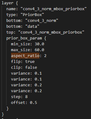
We can see that we will use aspect ratios 1, 1/2 and 2 for the stage 4 and 1, 1/2, 2, 1/3, 3 for the 7th. We also need to know the scale of each default box on the original image and the resolution of the feature map to know the number of boxes to create.
For instance, the stage 4 has a output resolution of 38×38 and aspect ratio of 2 (this means 1/2 and 2). We will have 4 boxes, the regular one of aspect ratio 1, the little one 0.5×0.5 and the aspect ratio 1/2 and 2. Each box will have 4 parameters for cx, cy, width and height. We should verify afterwards that we have 38x38x4 boxes and 38x38x4x4 numbers.
First, we will create the list of information needed:
self.ratios = [[1, 1/2, 2],
               [1, 1/2, 2, 1/3, 3],
               [1, 1/2, 2, 1/3, 3],
               [1, 1/2, 2, 1/3, 3],
               [1, 1/2, 2],
               [1, 1/2, 2]]
self.scales = [0.1, 0.2, 0.375, 0.55, 0.725, 0.9]
self.fm_resolutions = [38, 19, 10, 5, 3, 1]
Then, we can loop over these lists to create the boxes:
def getDefaultBoxes(self):
    boxes = []
    for fm_idx in range(len(self.fm_resolutions)):
        boxes_fm_i = []
        step = 1/self.fm_resolutions[fm_idx]
        for j in np.arange(0, 1, step):
            for i in np.arange(0, 1, step):
                # box with scale 0.5
                boxes_fm_i.append([i + step/2, j + step/2,
                                   self.scales[fm_idx]/2.,
                                   self.scales[fm_idx]/2.])
                # box with aspect ratio (1, 1/2, 2, 1/3, 3)
                for ratio in self.ratios[fm_idx]:
                    boxes_fm_i.append([i + step/2, j + step/2,
                                       self.scales[fm_idx] * np.sqrt(ratio),
                                       self.scales[fm_idx] / np.sqrt(ratio)])
         boxes.append(tf.constant((boxes_fm_i)))
    return boxes
Finally, we can get all the default boxes in the init() and display the resolutions of the list to verify the number of boxes:
self.default_boxes = self.getDefaultBoxes()
self.stage_4_boxes = self.default_boxes[0]
[...]
self.stage_11_boxes = self.default_boxes[5]

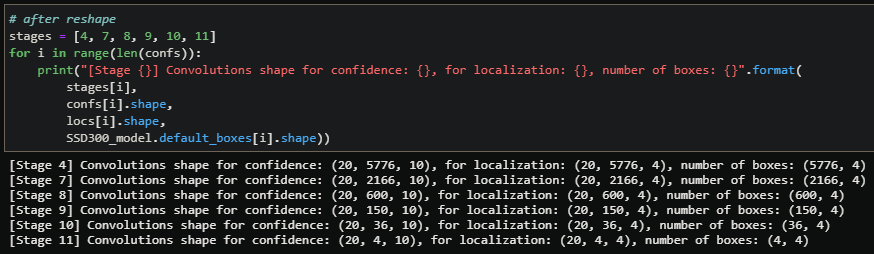
38x38x4=5776 and each box has 4 parameter. For the stage 8, there are 6 default boxes (1×1, 0.5×0.5, 1/2, 2, 1/3, 3) and 10x10x6=600. We can know notice an important thing: convolutions for localization of stage 4 equals 38x38x16=23,104, and the number of boxes parameters equals 5776×4=23,104! Finally, in this example we have 10 classes so we should have number of boxes times 10 number of convolution parameters for the confidence: 38x38x40/10=5776=number of boxes! This means that we will need to rescale the convolutions to fit the boxes representation (5776,4) to have the convolutions for confidence (5776, 10) and for localization (5776, 4):
Here is the function that reshape the confidence and loc convolutions output with the number of boxes, and the new resolutions:
def reshapeConfLoc(self, conf, loc, number_of_boxes):
    conf = tf.reshape(conf, [conf.shape[0], number_of_boxes, self.num_categories])
    loc = tf.reshape(loc, [loc.shape[0], number_of_boxes, 4])
    return conf, loc
All the network’s parameters are now set and have the good shape to be used.
3-4) Non-max suppression
The non-max suppression (NMS) used is described in the paper section 3.7:
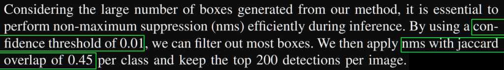
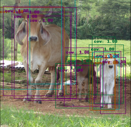
We will see in the next sections how to train the model and how to draw its results in images but I wanted to illustrate here the utility of NMS. The next animation shows the performance of the model we are building after a few epochs of training without NMS enabled:

The network found several boxes that match the actual object, which is true. However, this needs to be filtered to avoid having multiple detections of the same object. The method I implemented is a recursive NMS function that calls itself until there are no more overlapping boxes. It calculates an average box with all overlapping boxes of the same class and gets the maximum score. Note: the traditional NMS is a bit different, it normally keeps the box with the maximum IoU over all the other.
# loop over available classes
for category in tf.unique(classes)[0]:
    cat_idx = classes == category
    cat_boxes = boxes[cat_idx]
    cat_scores = scores[cat_idx]

    # compute mean boxes until there is no more overlapping boxes
    while cat_boxes.shape[0] != 0:
        iou = self.computeJaccardIdx(cat_boxes[0], cat_boxes, 0.3)
        not_iou = tf.math.logical_not(iou)

        overlap_scores = cat_scores[iou]
        iou = tf.expand_dims(iou, 1)
        iou = tf.repeat(iou, repeats=[4], axis=1)
        overlap_boxes = tf.reshape(cat_boxes[iou],
                                   (overlap_scores.shape[0], 4))
        mean_box = tf.math.reduce_mean(overlap_boxes, axis=0)
        filtered_boxes.append(mean_box)
        max_scores = tf.math.reduce_max(overlap_scores, axis=0)
        filtered_scores.append(max_scores)
        filtered_classes.append(category)

        # update available boxes with boxes without overlap
        cat_boxes = cat_boxes[not_iou]
        cat_scores = cat_scores[not_iou]

final_boxes = tf.convert_to_tensor(filtered_boxes, dtype=tf.float32)
final_classes = tf.convert_to_tensor(filtered_classes, dtype=tf.int16)
final_scores = tf.convert_to_tensor(filtered_scores, dtype=tf.float32)

# recursive call until no more overlap was found
if boxes_origin.shape != final_boxes.shape:
    final_boxes, final_classes, final_scores = \
        self.recursive_nms(final_boxes, final_classes, final_scores)
This produces the following result on the same example:

Other examples without and with NMS:


3-5) Losses
Thanks to the previous section, we know that we need to create losses for confidence and localization convolutions. The losses to use are described in the paper (section 2):

The Softmax loss means activation function Softmax plus a Cross-Entropy loss.
There is also a Negative Mining to implement: as there are many default boxes, we must discard the irrelevant ones to avoid having a vastnumber of negatives for a few positives. In the paper, they mentioned that we should not exceed 3:1 ratio between negatives and positives.
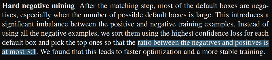
This means that we first need to calculates our loss for all the boxes, then sort them by confidence and finally select the (num_positives*3) negatives or less. Once we have calculated our loss for all the positives and selected negatives, we must divide them by the number of positives (N). If there are no positives, we set the loss to 0:

The last thing to know is that we use positives plus selected negatives for the confidence loss but only the positives for the boxes’ offsets regression:

An implementation could be the following one, but it may change once we are able to train the model:
def calculateLoss(self, confs_pred, confs_gt, locs_pred, locs_gt):
    """
    Method to calculate loss for confidences and localization offsets
    B = mini-batch size
    Args:
        - (tf.Tensor) confidences prediction: [B, N boxes, n classes]
        - (tf.Tensor) confidence ground truth:  [B, N boxes]
        - (tf.Tensor) localization offsets prediction: [B, N boxes, 4]
        - (tf.Tensor) localization offsets ground truth: [B, N boxes, 4]
    Return:
        - (tf.Tensor) confidences of shape [B, 1]
        - (tf.Tensor) loc of shape [B, 1]
    """
    positives_idx = confs_gt > 0
    positives_number = tf.reduce_sum(
        tf.dtypes.cast(positives_idx, self.floatType), axis=1)
    confs_loss_before_mining = self.before_mining_crossentropy(confs_gt,
                                                               confs_pred)

    # Negatives mining with <3:1 ratio for negatives:positives
    negatives_number = tf.dtypes.cast(positives_number, tf.int32) * 3
    negatives_rank = tf.argsort(confs_loss_before_mining, axis=1,
                                direction='DESCENDING')
    rank_idx = tf.argsort(negatives_rank, axis=1)
    negatives_idx = rank_idx <= tf.expand_dims(negatives_number, 1)

    # loss calculation (pos+neg for conf, pos for loc)
    confs_idx = tf.math.logical_or(positives_idx, negatives_idx)
    confs_loss = self.after_mining_crossentropy(confs_gt[confs_idx],
                                                confs_pred[confs_idx])

    locs_loss = self.smooth_l1(locs_gt[positives_idx],
                               locs_pred[positives_idx])

    confs_loss = confs_loss / tf.reduce_sum(positives_number)
    locs_loss = locs_loss / tf.reduce_sum(positives_number)

    return confs_loss, locs_loss
4) Database management
4-1) Read and parse annotations
To train our SSD model we need to preprocess data. We will use here the famous PASCAL VOC 2012 dataset for object detection and segmentation with 21 classes. This dataset contains 17,125 jpg images and annotations. There is an annotation per image with the following template:
<annotation>
    [some info about the image:
        filename, resolution, etc.]
    <object>
        <name>person</name>
        <truncated>0</truncated>
        <difficult>0</difficult>
        <bndbox>
            <xmin>100</xmin>
            <ymin>100</ymin>
            <xmax>150</xmax>
            <ymax>200</ymax>
        </bndbox>
        <part>
            <name>head</name>
            <bndbox>
                <xmin>110</xmin>
                <ymin>100</ymin>
                <xmax>130</xmax>
                <ymax>120</ymax>
            </bndbox>
        </part>
    </object>
</annotation>
For each annotation we can find the classes’ name under: annotation>object>name and for each object we also have access to the annotation of parts of the objects, like head for a person, under: annotation>object>part>name. then, we have the bounding box coordinate as (xmin, ymin, xmax, ymax) so we will need to convert it to (cx, cy, width, height). We will create a function that reads and parses an annotation file and returns the list of boxes and classes found:
def getAnnotations(self, image_name: str, resolution: tuple):
    """
    Method to get annotation: boxes and classes
    Args:
        - (str) image name without extension
        - (tuple) image resolution (W, H, C) or (W, H)
    Return:
        - (tf.Tensor) Boxes of shape: [number of objects, 4]
        - (tf.Tensor) Classes of shape: [number of objects]
    """
    boxes = []
    classes = []
    objects = ET.parse(
        self.annotations_path + image_name + ".xml").findall('object')
    for obj in objects:
        bndbox = obj.find('bndbox')
        xmin = float(bndbox.find('xmin').text) / resolution[0]
        ymin = float(bndbox.find('ymin').text) / resolution[1]
        xmax = float(bndbox.find('xmax').text) / resolution[0]
        ymax = float(bndbox.find('ymax').text) / resolution[1]

        # calculate cx, cy, width, height
        width = xmax-xmin
        height = ymax-ymin
        if xmin + width > 1. or ymin + height > 1. or\
            xmin < 0. or ymin < 0.:
            print("Boxe outside picture: (xmin, ymin, xmax, ymax):\
                  ({} {}, {}, {})".format(xmin, ymin, xmax, ymax))

        boxes.append([xmin+width/2., ymin+height/2., width, height])

        # get class
        name = obj.find('name').text.lower().strip()
        classes.append(self.classes[name])

    return tf.convert_to_tensor(boxes, dtype=self.floatType),\
        tf.convert_to_tensor(classes, dtype=tf.int16)
We can now create a function that returns the images, boxes and classes:
def getRawData(self, images_name: list):
    """
    Method to get images and annotations from a list of images name
    Args:
        - (list) images name without extension
    Return:
        - (tf.Tensor) Images of shape:
            [number of images, self.img_resolution]
        - (list of tf.Tensor) Boxes of shape:
            [number of images, number of objects, 4]
        - (list tf.Tensor) Classes of shape:
            [number of images, number of objects]
    """
    images = []
    boxes = []
    classes = []
    for img in images_name:
        image = tf.keras.preprocessing.image.load_img(
            self.images_path + img + ".jpg")
        w, h = image.size[0], image.size[1]
        image = tf.image.resize(np.array(image), self.img_resolution)
        images_array = \
            tf.keras.preprocessing.image.img_to_array(image) / 255.
        images.append(images_array)

        # annotation
        boxes_img_i, classes_img_i = self.getAnnotations(img, (w, h))
        boxes.append(boxes_img_i)
        classes.append(classes_img_i)
    return tf.convert_to_tensor(images, dtype=self.floatType),\
        boxes, classes
But this only returns the images in tensor format, the boxes (cx, cy, w, h) and corresponding classes. To train our neural network, we will need to convert these annotations to ground truth that respects the format of our default boxes seen in the previous section.
4-2) Create the ground truth from annotations
To convert the annotations to ground truth, we need to find which default box of the network is the closest to the one in the annotation. The term “closest” is defined by the Jaccard Overlap, in other words, by the intersection over union between the box in the annotations and a default box of the network. This Jaccard overlap is defined as:

This can be illustrated as follows for two boxes:

We first need a function that calculate the intersection over union, then, a function that processes the intersection over union between a box in the annotation and all the default boxes of the network. Instead of taking the one with the highest value, we take all the default boxes with IoU > 0.5. This is more comfortable for the network to learn because it has multiple choices. This is written in the paper section 2.2:
4-2-a) Unoptimized version
The first version I made was only a first simple approach. It uses many for loop and is not optimized at all. To compute our ground truth we need to:
- get the images, all the boxes for each image and their class
- compute the IoU between each box (often multiple boxes per image) and the 8732 default boxes of the network
- create a new tensor with value 0 if the IoU is under 0.5, we put the class number of the corresponding box otherwise
- compute the offsets between the ground truth and the matching default boxes (cx, cy, w, h)
These steps can be done as follows:
 images, boxes, classes = self.getRawData(images_name)
 gt_confs = []
 gt_locs = []
 for i, gt_boxes_img in enumerate(boxes):
    gt_confs_per_default_box = []
    gt_locs_per_default_box = []
    for d, default_box in enumerate(default_boxes):
        for g, gt_box in enumerate(gt_boxes_img):
            iou = self.computeJaccardIdx(gt_box, default_box)
            gt_conf = self.classes['undefined']
            gt_loc = tf.Variable([0.0, 0.0, 0.0, 0.0])
            if iou >= 0.5:
                gt_conf = tf.Variable(classes[i][g])
                gt_loc = self.getLocOffsets(gt_box, default_box)
        gt_confs_per_default_box.append(gt_conf)
        gt_locs_per_default_box.append(gt_loc)
    gt_confs.append(gt_confs_per_default_box)
    gt_locs.append(gt_locs_per_default_box)
In this version, there are 3 for loop and a if statement and my functions to compute the Jaccard Index and the offsets only take as input two single boxes (implementation of these two functions are available on my github). This version was too slow to be used. It takes 132s on my computer to compute the ground truth for a single image:

But that was not hard to optimize by doing all the computation of the tensors directly, instead of using a single element at a time.
4-2-b) Optimized version
This new optimized version was more efficient by doing the computation on the tensors:
 images, boxes, classes = self.getRawData(images_name)
 gt_confs = []
 gt_locs = []
 for i, gt_boxes_img in enumerate(boxes):
     gt_confs_per_image = tf.zeros([len(default_boxes)], tf.int16)
     gt_locs_per_image = tf.zeros([len(default_boxes), 4],
                                   self.floatType)
     iou_bin_masks = []
     for g, gt_box in enumerate(gt_boxes_img):
         iou_bin = self.computeJaccardIdxSpeedUp(gt_box,
                                                 default_boxes,
                                                 0.5)
         for mask in iou_bin_masks:
             iou_bin = tf.clip_by_value(iou_bin - mask, 0, 1)
             iou_bin_masks.append(iou_bin)
             gt_confs_per_image = gt_confs_per_image +\
                 iou_bin * classes[i][g]
             gt_locs_per_image = gt_locs_per_image +\
                 self.getLocOffsetsSpeedUp(gt_box, iou_bin, default_boxes)
     gt_confs.append(gt_confs_per_image)
     gt_locs.append(gt_locs_per_image)
We deleted the worst for loop. Thanks to it, we no longer loop over the 8732 defaults boxes, which should save us a considerable amount of time. We also removed the if statement to work with indexes from the new computeJaccardIdxSpeedUp() method. This new method and the new getLocOffsetsSpeedUp() takes as input the default boxes tensor, instead of using only a single box. All calculations are now performed directly on the tensors and here is the new processing time:
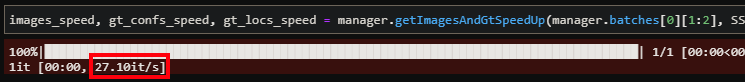
132 s/item to 27 items per s! It means that now it takes 0.036s per item so we divided the process time by 3,667 times.
We could do more optimization because if we want to load the whole dataset, it will take: 17125 images * 0.036 = 616 s ~ 10 mn. But all of this data will not fit in the memory of my computer so I will load the data on the fly during the training. This means that with a batch size of 32, my function to get the ground truth will take 1.152s, which is insignificant compared to the epoch time so no more optimization is needed.
4-2-c) confs_gt and locs_gt verification
4-2-c-i) IoU and default boxes verification
We can now call each individual methods to verify the entire process. First, we need to get the raw data described in the section 4.1:

then we can calculate the indexes where the IoU is superior to 0.5:
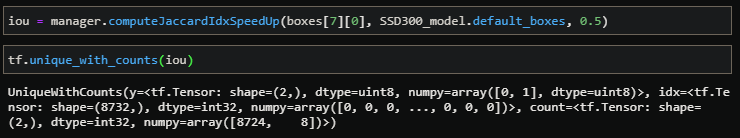
We can see that 8 default boxes has an IoU >= 0.5. Here is the actual gt box:

This is a big box because its width is 48% of the image width and its height 88% of the image height. We should match it with boxes at the bottom of the cone, where the feature maps are smaller. Plus, cx is 1/3 of the image and cy a bit more than 1/2 so we should match with boxes at the same location in the features maps. Here are the parameters for the feature maps:
self.ratios = [[1, 1/2, 2],
               [1, 1/2, 2, 1/3, 3],
               [1, 1/2, 2, 1/3, 3],
               [1, 1/2, 2, 1/3, 3],
               [1, 1/2, 2],
               [1, 1/2, 2]]
self.scales = [0.1, 0.2, 0.375, 0.55, 0.725, 0.9]
self.fm_resolutions = [38, 19, 10, 5, 3, 1]
We can see, thanks to the scale parameter, that the feature maps that should match the box are the 4th and the 5th. Then, here is how we get the default boxes:
boxes = []
for fm_idx in range(len(self.fm_resolutions)):
    boxes_fm_i = []
    step = 1/self.fm_resolutions[fm_idx]
    for j in np.arange(0, 1, step):
        for i in np.arange(0, 1, step):
            # box with scale 0.5
            boxes.append([i + step/2, j + step/2,
                self.scales[fm_idx]/2.,
                self.scales[fm_idx]/2.])
            # box with aspect ratio
            for ratio in self.ratios[fm_idx]:
                boxes.append([
                    i + step/2, j + step/2,
                    self.scales[fm_idx] / np.sqrt(ratio),
                    self.scales[fm_idx] * np.sqrt(ratio)])
We can notice that the order is always: ratio 0.5/0.5, ratio 1/1, ratio W/H 2/1, ratio W/H 1/3. So the last box is the one that looks like the original box of [0.293, 0.56, 0.78, 0.88] with Height greater than Width. If we pick the 5th feature map, we should get an IoU >= 0.5 at the following location:

This illustration shows how to verify the default boxes selected. We know that the original one has ratio width:height ~ 1:2 so the ratio of 1:1, 1:2 and 1:3 should match with an IoU>= 0.5 if they have their center at the good location. I have represented the original image in blue in the two feature maps selected. I have also mentioned the boxes number to know which number should have a good IoU. (Remark: the 6th and 5th have 4 default boxes and the 4th has 6). According to the location, the gt box should match with the boxes number 25 and 27 (starting from end), and 89, 91, 93, 119, 121 and 122 on the 4th feature map. We can verify it with the indexes of the IoU tensor calculated previously:

This is exactly what we get! We can see that we have 1 at the good location in the IoU tensor and only at this location because we saw previously that we got only 8 matches. We can assume that the IoU calculation was done correctly and the default boxes implementation too.
As a final verification we can create a code that displays the ground truth box from the annotations and the boxes and classes selected. Here I plot the ground truth in green and the default boxes selected + the class (available in the eval.py script):

The selected classes and default boxes seem perfect.
4-2-c-ii) Offsets verification
We can now verify for each box if the the offsets calculated were correct. Our ground truth box is the following one:
And here we can verify the offsets for the default boxes 119, 121, 123 starting from end:

The offsets are correct. Plus, if I use the previous code to draw the default boxes selected + the offsets, all the red rectangles come to the green one.
4-2-c-iii) ground truth confs and locs verification
We can now verify the class of the box 7th (the same one we took previously) and verify that we have the same class in gt_confs and the same offsets in gt_locs for the box -119 for instance:
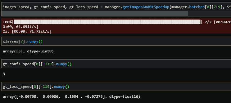
We got the same class in gt_conf and the same offsets in gt_locs, everything looks good. The same thing we can verify is if we got only 8 values different from 0 in gt_confs and gt_locs and at the good places:

We get exactly 8 values different from zero in gt_conf and gt_locs, we got only 0 and 3 for the gt_confs which is correct and we got all the offsets previously seen in the gt_locs.
5) Training
5-1) Load pre-trained weights
Before creating the function to train our model, we need to set up the environment described in the paper. In particular, it is mentioned in section 3 that the base network (VGG16) has been pre-trained on the ILSVRC CLS-LOC – ImageNet dataset:

Fortunately, we will not need to train it ourselves as Tensorflow supplies the VGG16 model with pre-trained weights on ImageNet. So all we must do is load this model with these weights and load them into our base network:
from tensorflow.keras.applications import VGG16 as VGG16_original
[...]

def load_vgg16_imagenet_weights(self):
    """ Use pretrained weights from imagenet """
    vgg16_original = VGG16_original(weights='imagenet')

# load weights from conv_1_1_64 to conv_4_3_512
for i in range(len(self.VGG16_stage_4.layers)):
    self.VGG16_stage_4.get_layer(index=i).set_weights(
        vgg16_original.get_layer(index=i+1).get_weights())

# load weights from maxpool_4_4_2x2 to conv_5_3_512
for j in range(len(self.VGG16_stage_5.layers)):
    self.VGG16_stage_5.get_layer(index=j).set_weights(
        vgg16_original.get_layer(index=i+j+2).get_weights())
5-2) Optimizer and gradient calculation from loss
SDD model has been training with SGD with initial learning rate of 10^-3 and 0.9 momentum was used. Finally, a weight decay and batch size = 32:

The following optimizer combines all information except the learning rate decay:
optimizer = tf.keras.optimizers.SGD(learning_rate=10**-3, momentum=0.9)
As the paper mentioned that the learning rate strategy changes with the dataset, we must look at the one used with our dataset Pascal VOC 2012. We can see it in the official code under docs/examples/ssd/ssd_pascal_orig.py:

We can implement it with the following code in TensorFlow:
from tensorflow.keras.optimizers.schedules import PiecewiseConstantDecay
init_lr = 0.001
lr_decay = PiecewiseConstantDecay(boundaries=[80000, 10000, 120000],
                                  values=[init_lr, 0.0005, 0.0001, 0.00005])
optimizer = tf.keras.optimizers.SGD(learning_rate=lr_decay, momentum=0.9)
5-3) Training function
A simple training function could be the following one:
- Loop over the epochs,
- Loop over the batches,
- Get the data: images, confs_gt and locs_gt
- Infer the model on the images and get the confs_pref and locs_pred
- Calculate the loss
- Do back propagation
- Save the model weights every N epochs
for epoch in range(num_epoch):
        losses = []
        for i in tqdm(range(len(imgs))):
            # get data from batch
            images, confs_gt, locs_gt = imgs[i], confs[i], locs[i]

            # get predictions and losses
            with tf.GradientTape() as tape:
                confs_pred, locs_pred = model(images)
                # concat tensor to delete the dimension of feature maps
                confs_pred = tf.concat(confs_pred, axis=1)
                locs_pred = tf.concat(locs_pred, axis=1)

                # calculate loss
                confs_loss, locs_loss = model.calculateLoss(
                    confs_pred, confs_gt, locs_pred, locs_gt)
                loss = confs_loss + 1*locs_loss  # alpha equals 1
                l2 = [tf.nn.l2_loss(t)
                      for t in model.trainable_variables]
                loss = loss + 0.001 * tf.math.reduce_sum(l2)
                losses.append(loss)

            # back propagation
            gradients = tape.gradient(loss, model.trainable_variables)
            optimizer.apply_gradients(
                zip(gradients, model.trainable_variables))
        print("Mean loss: {} on epoch {}".format(np.mean(losses), epoch))
        if epoch % inter_save == 0:
            model.save_weights(weights_path +
                               "/ssd_weights_epoch_{:03d}.h5".format(epoch))
6) Get model’s results
6-1) Draw predictions and ground truth on images
To print the predicted boxes and ground truth we need two functions:
- A function to select the predicted boxes in function of a confidence threshold and filter the one with undefined class
- A second function to draw boxes on an image
The first function can filter the predicted boxes (confidence threshold and undefined class removal) with few lines:
# SSD model predict offsets to add to default boxes
# To get the predicted boxes we need to add these offsets to the default boxes
boxes = self.default_boxes + locs_pred[i]

# get the indexes of the boxes with at least score_threshold value
scores = tf.reduce_max(confs_pred[i], axis=1)
idx_sup_thresh = scores >= score_threshold

# Get indexes within the 21 classes to filter the ones with 0 (undefined) class
classes = tf.argmax(confs_pred[i], axis=1)
non_undefined_idx = classes > 0

# combine both indexes
idx_to_keep = tf.logical_and(idx_sup_thresh, non_undefined_idx)
classes = classes[idx_to_keep]
boxes = boxes[idx_to_keep]
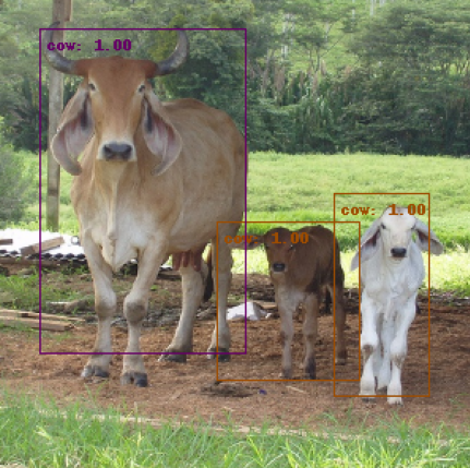
As our ground truth boxes are already in a good shape, we just need to draw them without any preprocessing. The second function to draw the boxes in an image is available on my Github under eval.py script. Here are some results for the default boxes selected in red and the ground truth boxes in green:

6-2) Draw predictions on video
We can also use the same code to print predictions on a video. We only need a few lines of code to load the video and then infer the network on each image. The function can be found in utils/eval.py: pltPredOnVideo() and can be used as follows:
pltPredOnVideo(SSD300_model, db_manager, video_path, out_path + "my_gif.gif")


Note: it could be good to add labels smoothing techniques in SSD training because the network seems too confident with the classes
Conclusion:
This implementation allowed me to understand in depth how object detection using deep learning algorithms can be achieved. I hope this article will help others.
The next steps will be a module to do multi-object tracking (MOT) and use the SSD300’s predictions as box proposal.
Here you can find my project:
https://github.com/Apiquet/Tracking_SSD_ReID
Video source: coveer
