

SLAM: Simultaneous Localization and Mapping: Mathematical foundations
This series of articles is an introduction to SLAM algorithm and can be seen as a summary of the SLAM resources given on the following repository. Some good illustrations that help to understand the concepts will be displayed, some are come from their pdf document.
This article first briefly introduces SLAM problems and then focuses on the mathematical foundations needed to solve them: coordinate manipulation (vectors, rotation matrix, quaternion, etc.) and transformations (similarity and perspective).
Table of contents
- Introduction
- SLAM framework overview
- Maps types
- Mathematical formulation of SLAM problems
- General formulation
- Linear Gaussian (LG system) and Gaussian/non-Gaussian systems
- Coordinate manipulation
- Vector operations
- Euclidean Transforms
- Rotation matrix
- Translation matrix
- Transform matrix
- Rotation vector
- Euler angles
- Quaternion
- Quaternion operations
- Quaternion to represent a rsotation
- Transformations
- Similarity transformation
- Perspective transformation
- Summary
1) Introduction
SLAM stands for Simultaneous Localization and Mapping. It usually refers to a robot or a moving rigid body, equipped with a specific sensor, estimates its motion and builds a model (certain kinds of description) of the surrounding environment, without a priori information. If the sensor referred to here is mainly a camera, it is called Visual SLAM.
SLAM aims at solving the localization and map building issues at the same time. In other words, it is a problem of how to estimate the location of a sensor itself, while estimating the model of the environment.
If the main sensor used is a camera, then we talk about Visual SLAM.
Camera can be a different types:
- Monocular camera: only one camera
- Advantages: simple sensor, low cost
- Inconvenient: The absolute distance of the objects remains unknown. We can only estimate the relative distance between objects using parallax (distant objects will have a smaller displacement in the image than closer objects).
The trajectory and map obtained from monocular SLAM estimation will differ from the actual trajectory and map with an unknown factor, which is called the scale. Since monocular SLAM can not determine this real scale purely based on images, this is also called the scale ambiguity.
- Stereo Cameras and RGB-D Cameras
- Advantages: the absolute distance can be known:
- A stereo camera consists of two synchronized monocular cameras, displaced with a known distance, namely the baseline. Because the physical distance of the baseline is known, we can calculate each pixel’s 3D position in a very similar way to our human eyes. Stereo matching consume many computational resources
- Depth camera (RGB-D camera): Similar to laser scanners, RGB-D cameras adopt infrared structure of light or Time-of-Flight (ToF) principles and measure the distance between objects and the camera by actively emitting light to the object and receive the returned light. This part is not solved by software as a stereo camera, but by physical sensors to save many computational resources compared to stereo cameras
- Inconvenient: more expensive, configuration and calibration process, the depth is also: noisy (both), small field of view (RGB-D), susceptibility to sunlight interference (both), unable to measure transparent material (both), wrong distance on reflective surface like mirrors (stereo)
- Advantages: the absolute distance can be known:
2) SLAM framework overview
The classic visual SLAM framework is composed of:
- Sensor data acquisition: acquisition and preprocessing of camera images,
- Visual Odometry (VO) named as frontend: estimate the camera movement between adjacent frames (ego-motion) and generate a rough local map,
- Backend filtering/optimization: receives camera poses at different time stamps from VO and results from loop closing, and then applies optimization to generate a fully optimized trajectory and map. It mainly refers to the process of dealing with the noise in SLAM systems,
- Loop Closing: determines whether the robot has returned to its previous position in order to reduce the accumulated drift. If a loop is detected, it will provide information to the backend for further optimization,
- Reconstruction: task-specific map based on the estimated camera trajectory.

3) Maps types
The map built by SLAM algorithms can be of different types:
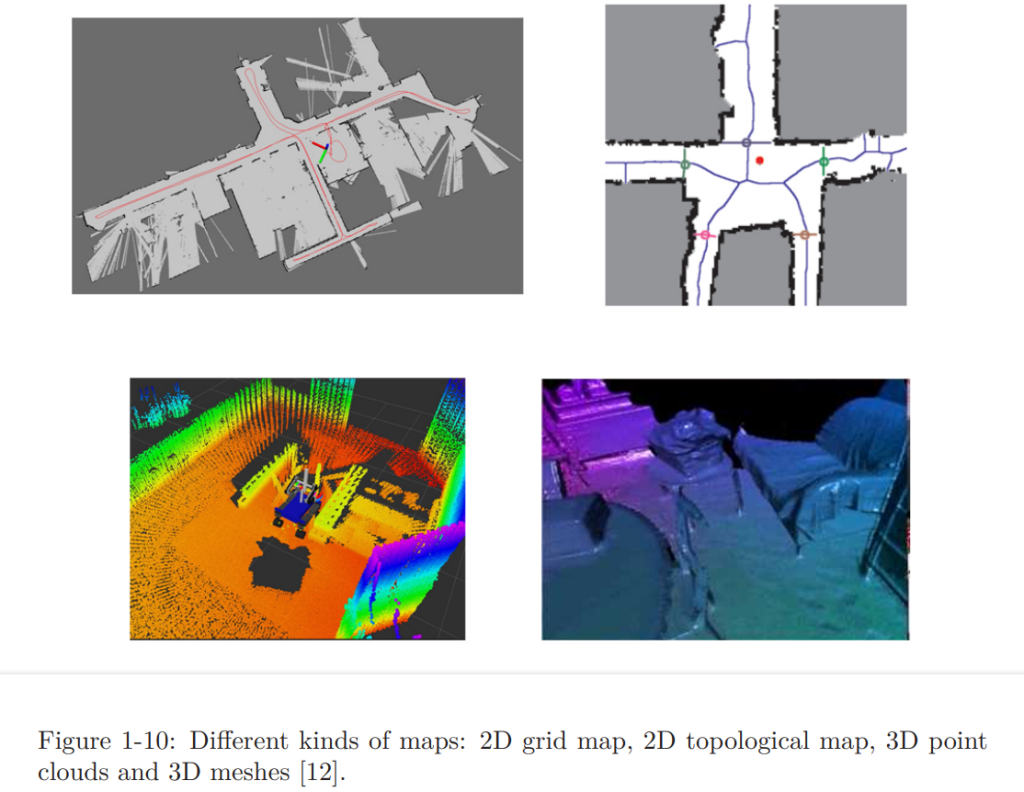
There are mainly two categories, metrical maps and topological maps:
- Metrical maps: emphasize the exact metrical locations of the objects in maps either sparse or dense. Contrary to dense maps, sparse maps does not express all the objects (for a road: only lanes and traffic signs for instance).
A dense map usually consists of a number of small grids at a certain resolution. It can be small occupancy grids for 2D metric maps or small voxel grids for 3D maps. A grid may have three states: occupied, not occupied, and unknown, to express whether there is an object. - Topological maps: emphasize the relationships among map elements. A topological map is a graph composed of nodes and edges, only considering the connectivity between nodes.
4) Mathematical formulation of SLAM problems
4-1) General formulation
If a robot moves in a plane, then its pose is described by two x − y coordinates and an angle, i.e., xk = [x1, x2, θ], where x1, x2 are positions on two axes and θ is the angle. The motion equation can be parameterized as:
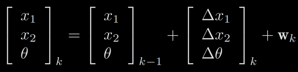
However, not all input commands are position and angular changes. For example, the input of “throttle” or “joystick” is the speed or acceleration, so there are other forms of more complex motion equations.
For example, if the robot carries a two-dimensional laser sensor which observes a 2D landmark by measuring: the distance r between the landmark point and the robot, and the angle ϕ. Let’s say the landmark is at yj = [y1, y2], the pose is xk = [x1, x2], and the observed data is zk,j = [rk,j , ϕk,j], then the observation equation is written as:
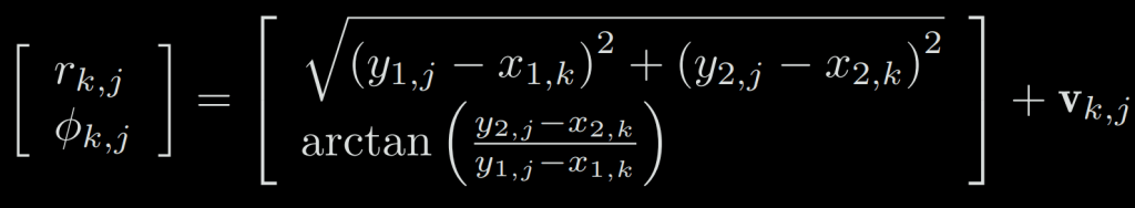
When considering visual SLAM, the sensor is a camera, then the observation equation is a process like “getting the pixels in the image of the landmarks.” This process involves a description of the camera model, which will be covered in detail later.
If we maintain versatility and take them into a common abstract form, then the SLAM process can be summarized into two basic equations:

where f() is the motion equation with x a landmark position, u the input command and w the noise, g() is the observation equation with a landmark point y at x and noise v to generate an observation z.
O is a set that contains the information at which pose the landmark was observed (usually not all the landmarks can be seen at every moment – we are likely to see only a small part of the landmarks at a single moment).
These two equations together describe a basic SLAM problem: how to solve the estimate x (localization) and y (mapping) problem with the noisy control input u and the sensor reading z data? Now, as we see, we have modeled the SLAM problem as a state estimation problem: How to estimate the internal, hidden state variables through the noisy measurement data?
The solution to the state estimation problem is related to the two equations’ specific form and the noise probability distribution. Whether the motion and observation equations are linear and whether the noise is assumed to be Gaussian, it is divided into linear/nonlinear and Gaussian/non-Gaussian systems.
4-2) Linear Gaussian (LG system) and Gaussian/non-Gaussian systems
The Linear Gaussian (LG system) is the simplest, and its unbiased optimal estimation can be given by the Kalman Filter (KF). In the complex nonlinear non-Gaussian (NLNG system), we basically rely on two methods: Extended Kalman Filter (EKF) and nonlinear optimization.
The mainstream of visual SLAM uses state-of-the-art optimization techniques represented by graph optimization. We believe that optimization methods are clearly superior to filters, and as long as computing resources allow, optimization methods are often preferred.
4-3) Coordinate manipulation
4-3-a) Vector operations
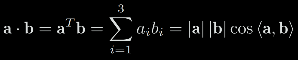
In a usual 3D space, we will work with 3D vectors to describe a simple point in space. This vector will then have to be transformed according to the necessary calculations. These calculations can be: addition, subtraction, inner product, outer product, etc.
It is important to be familiar with all these kind of transformations. For instance:
Inner product describes the projection relationship between vectors:
The result of the outer product is a vector whose direction is perpendicular to the two vectors, and the length is |a|.|b|.sin<a, b>, which is also the area of the quadrilateral of the two vectors.
The ^ operator means writing a as a skew-symmetric matrix:

4-3-b) Euclidean Transforms
The Euclidean transform consists of rotation and translation of a rigid object.
4-3-b-i) Rotation matrix
Let’s first assume we have two unit-length orthogonal bases (e1, e2, e3) and (e1′, e2′, e3′) corresponding to a simple rotation. Then, for a vector a, its coordinates in these two coordinate systems will be [a1, a2, a3] and [a1′, a2′, a3′]. Because the vector itself has not changed, according to the definition of coordinates, there are:
This leads to the following equation after a multiplication with transposed e:
This R matrix consists of the inner product between the two sets of bases. Since the base vector’s length is 1, it is also called direction cosine matrix.
The rotation matrix has some special properties. In fact, it is an orthogonal matrix (a square matrix whose columns and rows are orthonormal vectors) with a determinant of 1 (preserve volume).
4-3-b-ii) Translation matrix
The translation matrix is simply added after the rotation. To transform the coordinates of system 2 into 1, we write :
4-3-b-iii) Transform matrix
With the previous formula, passing from point a to point b will become b = R1.a + t1 and b to c: c = R2.b + t2 then passing from a to c: c = R2(R1.a + t1) + t2
To solve this problem, the transformation matrix was introduced, combining rotation and translation into a single matrix:
4-3-c) Rotation vector
The rotation matrix has few inconvenient:
- It uses 9 quantities to represent only a 3D rotation of 3 degrees of freedom,
- The transformation matrix then have 16 quantities for a 6 degrees of freedom (3 for rotation + 3 for translation),
- It has two major constraints: orthogonal and det=1 which makes harder the estimation and optimization process.
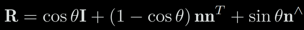
However, to represent a rotation, we can only use a 3D vector parallel to the axis of rotation and whose length is equal to the angle. This is called the rotation vector.
The conversion from the rotation vector to the rotation matrix is shown by the Rodrigues’ formula:
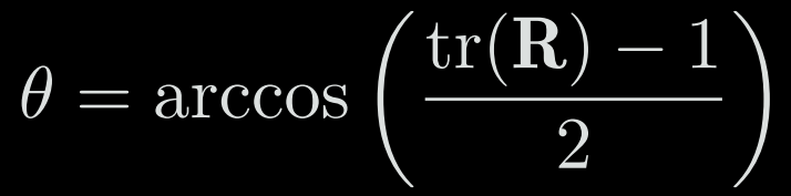
We also get the rotation angle with:
4-3-d) Euler angles
Contrary to the rotation matrix/vector, the Euler angle provides a very intuitive way to describe the rotation. It uses three primal axes to decompose a rotation into three rotations around different axes. However, due to the variety of decomposition methods, there are many alternative and confusing definitions of Euler angles. For example, we can first rotate around the X axis, then the Y axis, and finally around the Z axis, and in this way, we get a rotation like XY Z order. Similarly, you can define rotation orders such as ZYZ and ZYX. You also need to distinguish whether it is rotated around the fixed axis or around the axis after rotation, which will also give a different definition.
The commonly used order is ZYX also named ypr for Yaw Pitch Roll.
A major drawback of Euler Angle is that it encounters the famous Gimbal lock. With the ypr order, it appears when pitch=+/-90°. In theory, it can be proved that as long as you want to use three real numbers to express the three-dimensional rotation, you will inevitably encounter this singularity problem.
Note: If you are not familiar with gimbal lock, please see a video online that explains it as it will be easier to understand through animations.
Due to this fact, Euler angles are rarely used to express poses directly in the SLAM program. However, if you want to verify that your algorithm is correct or not, converting to Euler angles can help you quickly determine if the results are correct or not.
4-3-e) Quaternion
Quaternions are extended complex numbers, compact and not singular (contrary to euler angles). If we want to rotate the vector of a complex plane by θ, we can multiply this complex vector by exp(iθ) = cos(θ) + i.sin(θ).
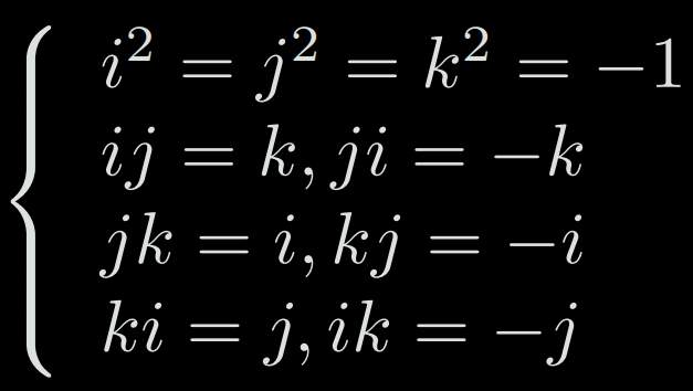
A quaternion q has a real part and three imaginary parts: q = q0 + q1.i + q2.j + q3.k with the relationships:
4-3-e-i) Quaternion operations
To multiply two quaternion, we multiply all elements of the first quaternion with all the elements of the second one:
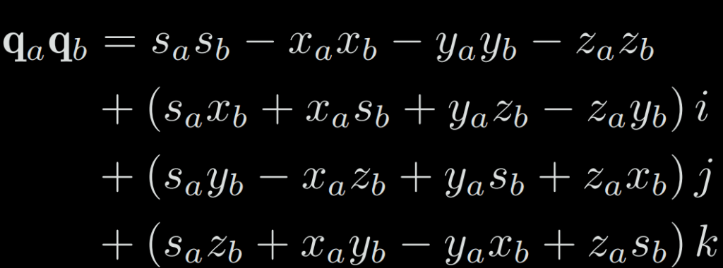
We can also describe this multiplication with the vector form:

Note that a multiplication of quaternions is generally not commutative (q1q2 != q2q1) unless they are parallel (because of the last term which is an outer product: axb=|a|b|cos(a, b)).
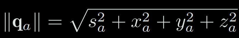
The length of a quaternion is defined as:
The conjugate of a quaternion is the opposite of the imaginary part: q*= s – x1 -yj – zk = [s, -v]
q*q is a real quaternion: q*q = qq* = [s² + transposed(v)v, 0]
The inverse of a quaternion is q* / (||q||²) and inv(q).q = 1
4-3-e-ii) Quaternion to represent a rotation
To rotate a 3D point p=(x, y, z) with a quaternion, we create a new quaternion as [0, x, y, z] so the real part is 0. Then, we compute : p’ = q.p.inv(q)
4-4) Transformations
4-4-a) Similarity transformation
The similarity transformation has one more degree of freedom than the Euclidean transformation, which allows the object to be uniformly scaled.
4-4-b) Perspective transformation
The perspective transformation is the most general transformation. The transformation from the real world to a camera photo can be seen as a perspective transformation. For instance, if we image a square tile in a photo: first, it is no longer square. Second, since the close part is larger than the far-away part, it is not even a parallelogram but an irregular quadrilateral.
4-4-c) Summary
We will introduce later that the transformation from the real world to the camera photo is a perspective transformation. If the focal length of the camera is infinity, then this transformation is affine.
The next article will go deeper into the comprehension of concepts such as Lie Group / Lie Algebra, Camera representation and non-linear optimizations.
