Computer Vision, SLAM

SLAM: Simultaneous Localization and Mapping: Theoretical part

This series of articles is an introduction to SLAM algorithm and can be seen as a summary of the SLAM resources given on the following repository. Some good illustrations that help to understand the concepts will be displayed, some are come from their pdf document.

This article will go deeper into the comprehension of concepts such as Lie Group / Lie Algebra, Camera representation and non-linear optimizations.

Table of contents

1. Lie Group and Lie Algebra
   1. Group
   2. Lie Group
   3. Lie Algebra
   4. Lie Algebra Derivation and Perturbation Model
      1. Derivation
      2. Derivative model
      3. Perturbation model
2. Cameras and Images: Pinhole Camera Model
   1. Intrinsics
   2. Extrinsics
   3. Distortion model
   4. Stereo cameras
   5. RGB-D Cameras
3. Nonlinear Optimization
   1. State Estimation
      1. From Batch State Estimation to Least-square
      2. Introduction to Least-squares
   2. Nonlinear Least-square Problem
      1. The First and Second-order Method
      2. The Gauss-Newton Method
      3. The Levernberg-Marquatdt Method
4. Conclusion

1) Lie Group and Lie Algebra

Because the pose is unknown in SLAM, we need to solve the problem of which camera pose best matches the current observation. A typical way is to build it into an optimization problem, solving the optimal R,t and minimizing the error.

The rotation matrix itself is a constrained (orthogonal, and the determinant is 1) matrix. When used as optimization variables, it introduces additional constraints on matrices that make optimization difficult. Through the transformation relationship between Lie group and Lie algebra, we can turn the pose estimation into an unconstrained optimization problem and simplify the solution.

1-1) Group

A group is an algebraic structure of one set plus one operator. We denote the set as A and the operation as ·, then the group can be denoted as G = (A, ·). We say G is a group if the operation satisfies the following conditions:

For instance, the three-dimensional rotation matrix in the special orthogonal SO(3) is a group with the multiplication operation and the addition of integers is also a group.

1-2) Lie Group

Lie Group refers to a group with continuous (smooth) properties.

Discrete groups like the integer group Z have no continuous properties, so they are not Lie groups. And obviously, SO(n) and SE(n) are continuous in real space because we can intuitively imagine that a rigid body moving continuously in the space, so they are all Lie Groups.

1-3) Lie Algebra

Each Lie group has a Lie algebra corresponding to it. Lie algebra describes the local structure of the Lie group around its origin point, or in other words, is the tangent space. The general definition of Lie algebra is listed as follows:

The binary operations [, ] are called Lie brackets. At first glance, we require a lot of properties about the Lie bracket. Compared to the simpler binary operations in the group, the Lie bracket expresses the difference between the two elements. It does not require a combination law but requires the element and itself to be zero after the brackets. For example, the cross product × defined on the 3D vector R3 is a kind of Lie bracket, so g = (R3, R, ×) constitutes a Lie algebra.

1-4) Lie Algebra Derivation and Perturbation Model

A major motivation for using Lie algebra is to do optimization. The derivative is a very necessary part of the optimization process.

First, we have already understood the relationship between Lie group and Lie algebra. Let’s take an example:

ln(exp(A)exp(B)) = A + B is unfortunatly not true for matrix. The complete form of the product is given by the Baker-Campbell-Hausdorff formula (BCH formula):

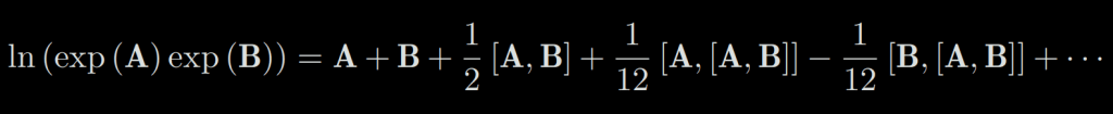
where [] is the Lie brackets. The BCH formula tells us that how to deal with the product of two matrices: they produce some extra Lie brackets compared with the scalar form.

BCH has a linear approximation:

Suppose we have a rotation R, the corresponding Lie algebra is ϕ. We give it a small perturbation to the left, denoted as ∆R, and so that the corresponding Lie algebra is ∆ϕ. Then, on Lie group, the result is ∆R · R, and on the Lie algebra, according to the BCH approximation, it is J−1 l (ϕ)∆ϕ + ϕ. Putting them together, we can simply write:

1-4-1) Derivation

Now let’s talk about how to compute the derivation if our target function is related to a rotation or a transform, which has a powerful practical meaning since we usually have these functions to optimize in solving the SLAM problem. Assume we want to estimate a pose described by SO(3) or SE(3) elements. Our robot observes a point with the world coordinate p and generates an observation data z, which can be written as: z = Tp + w, with w the noise.

Suppose we have N points in total, then we find a best T to make the error minimized:

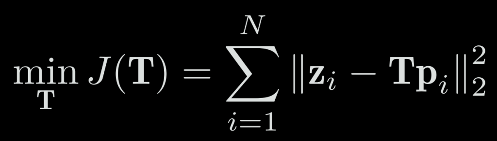
Because of the noise, the real observed data is not absolutely the same as the one we computed from the observation model, so we can calculate the error of predicted observation with the real one: To solve such an optimized problem (which is a least square problem), we need to calculate the derivative of J and T.

We have to adjust those rotations or transforms to find a better/best estimation. But, as we mentioned before, since SO(3) and SE(3) do not have a well-defined addition (they are just groups), so the derivatives cannot be defined in their common form. If we treat the R or T as common matrices, we have to introduce the constraints into our optimization.

However, from the perspective of Lie algebra, since it consists of vectors, it has a good addition operation. Therefore, there are two ways to solve the problem of derivation using Lie algebra:

• Assume we add a infinitesimal amount on Lie algebra, then compute the change of the object function,
• Assume we multiply an infinitesimal perturbation on the Lie group left multiplication or right multiplication, use Lie algebra to describe the perturbation, and then compute the derivative on this perturbation. This is called as left perturbation or right perturbation model.

The first method corresponds to the normal derivation model of the Lie algebra, and the second corresponds to the perturbation model. Let’s discuss the similarities and differences between these two approaches.

1-4-2) Derivative model

First, consider the situation on SO(3). Suppose we rotate a space point p and get Rp. To calculate the derivative of the point coordinates by the rotation, we informally write it as:

Since SO(3) has no addition operator, it cannot be calculated by the common derivative definition. Let the Lie algebra corresponding to R be ϕ, and we will calculate instead of the common derivative:

.
The second line is BCH approximation. The third line is Taylor’s approximation after throwing the high-order terms (but we still write the equal sign here because the limit is taken). The fourth to the fifth line treat the skew-symmetric symbol a cross-product so that a × b = −b × a. Thus, we compute the derivative of the rotated point relative to the addition in Lie algebra:

However, since there is still a very complicated form of J, we don’t want to calculate it. The perturbation model described below provides a more straightforward way to compute derivatives.

1-4-3) Perturbation model

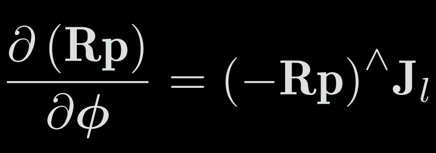
Another way to do this is to perturb R by ∆R and see the change of the result relative to the disturbance. This disturbance can be multiplied on the left or on the right. The final result will be slightly different. Let’s take the left perturbation as an example. Let the left perturbation ∆R correspond to the Lie algebra as φ. Then, for φ, that is:

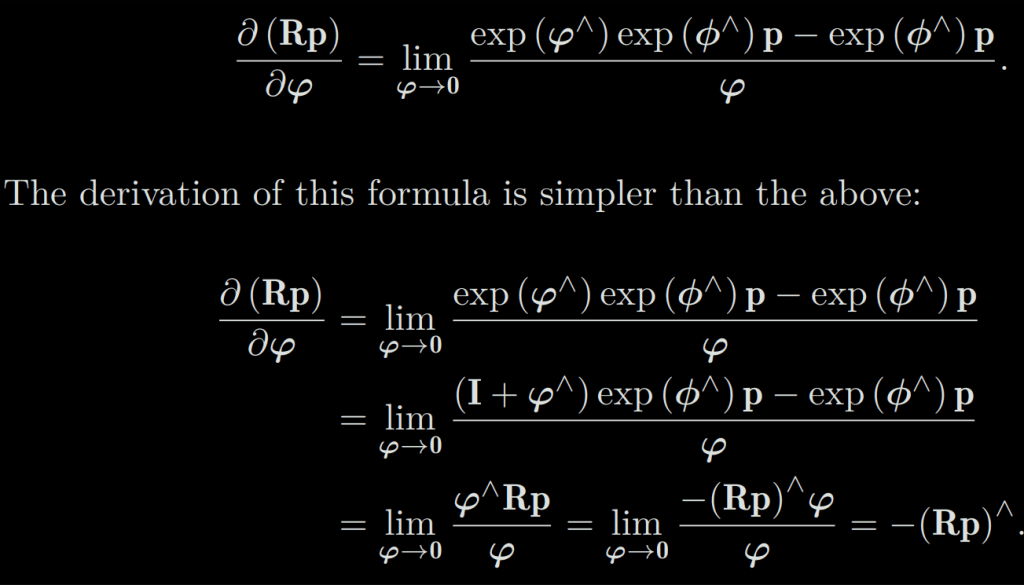
It can be seen that the calculation of a Jacobian J is omitted compared to Lie algebra’s direct derivation. This makes the perturbation model more practical.

Suppose a point p is transformed by T (corresponding to Lie algebra ξ), and the result is Tp^8. Now, give T a left perturbation ∆T = exp (δξ ∧), whose Lie algebra is δξ = [δρ, δϕ], then:

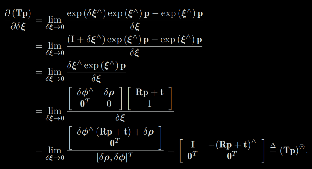
We define the final result as an operator ⊙9, which transforms a spatial point of homogeneous coordinates into a matrix of 4 × 6. This equation requires a little explanation about matrix differentiation. Assuming that a, b, x, y are column vectors, then in our book, there are following rules:

Substituting this into the last line, you can get the final result. So far, we have introduced the differential operation on Lie group Lie algebra. In the following chapters, we will apply this knowledge to solve practical problems.

2) Cameras and Images: Pinhole Camera Model

This section will discuss “How robots observe the outside world”, which belongs to the observation equation. In the camera-based visual SLAM, the observation mainly refers to the process of image projection.

The process of projecting a 3D point (in meters) to a 2D image plane (in pixels) can be described by a geometric model. Actually, several models describe this, the simplest of which is called the pinhole model. Due to the presence of the lens on the camera lens, a distortion model will also be used.

Here is an illustration of the model to explain the camera’s imaging process:

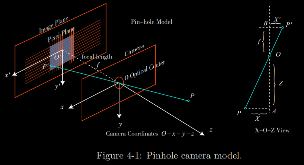
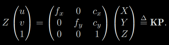
The next formula describes the spatial relationship between the point P and its image, where the units of all points are meters. For example, a focal length maybe 0.2 meters, and X′ be 0.14 meters. However, in the camera, we end up with pixels, where we need to sample and quantize the pixels on the imaging plane. To describe how the sensor converts the perceived light into image pixels, we set a pixel plane o − u − v fixed on the physical imaging plane. Finally, we get pixel coordinates of P’, in the pixel plane: [u, v]^T:

2-1) Intrinsics

In the next equation, we refer to the matrix composed of the middle quantities as the camera’s inner parameter matrix (o intrinsics) K. It is generally assumed that the camera’s internal parameters are fixed after manufacturing and will not change during usage. Some camera manufacturers will tell you the intrinsics, and sometimes you need to estimate the internal parameters by yourself, which is called calibration:

2-2) Extrinsics

In the previous equation, we use the coordinates of P in the camera coordinate system, but in fact, the coordinates of P should be its world coordinates because the camera is moving (we use the symbol Pw). It should be converted to the camera coordinate system based on the current pose of the camera. The camera’s pose is described by its rotation matrix R and the translation vector t:

The camera’s pose R,t is also called the camera’s extrinsics. Compared with the intrinsic, the extrinsics may change with the camera installation and is also the target to be estimated in the SLAM if we only have a camera.

2-3) Distortion model

In order to get a larger FoV (Field-of-View), we usually add a lens in front of the camera. The addition of the lens has an influence on the propagation of light during imaging: (1) the shape of the lens may affect the propagation way of light, (2) during the mechanical assembly, the lens and the imaging plane are not entirely parallel, which also changes the projected position.

There are two main categories:

The final model with 5 distortion coefficients is:

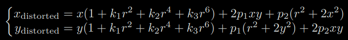
Please see the book for the complete explanation.

2-4) Stereo cameras

The pinhole camera model describes the imaging model of a single camera. However, we cannot determine the specific location of a spatial point only by a single pixel. This is because all points on the line from the camera’s optical center to the normalized plane can be projected onto that pixel. Only when the depth of P is determined (such as through a binocular or RGB-D camera) can we know exactly its spatial location.

There are many ways to measure the pixel distance (or depth). For example, the human eye can judge the object’s distance according to the difference (or parallax) of the scene seen by the left and right eyes. The binocular camera principle is also the same.

A binocular camera is generally composed of a left-eye camera and a right-eye camera. They are synchronized and placed horizontally, meaning that both cameras’ centers are on the same x axis. The distance between the two centers is called baseline (denoted as b), which is an important parameter:

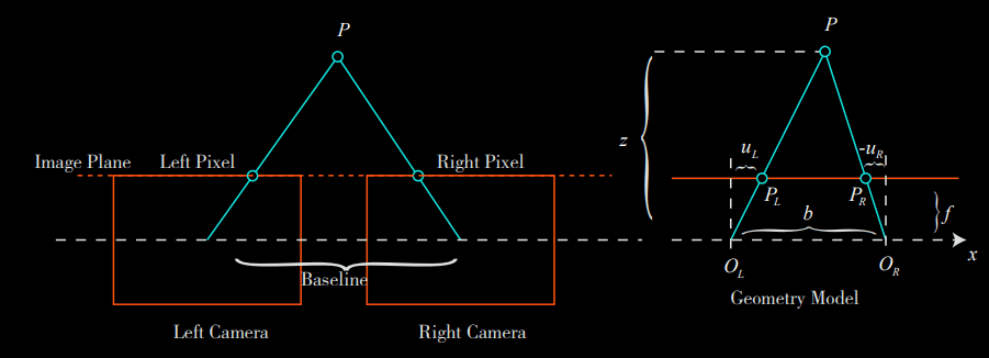
Now consider a 3D point P, projected into the left-eye and the right-eye, written as PL, PR. Due to the presence of the camera baseline, these two imaging positions are different. Ideally, since the left and right cameras are only shifted on the x axis, the image of P also differs only on the x axis (corresponding to the u axis of the image). Take the left pixel coordinate as uL and the right coordinate as uR:

2-5) RGB-D Cameras

Compared to the binocular camera’s way of calculating depth, the RGB-D camera’s approach is more “active”: it can actively measure each pixel’s depth. The current RGB-D cameras can be divided into two categories according to their principle:

1. The first kind of RGB-D sensor uses structured infrared light to measure pixel distance. Many of the old RGB-D sensors are belong to this kind, for example, the Kinect 1st generation, Project Tango 1st generation, Intel RealSense, etc.
2. The second kind measures pixel distance using the time-of-flight (ToF). Examples are Kinect 2 and some existing ToF sensors in cellphones

3) Nonlinear Optimization

Due to the presence of noise, the equations of motion and observation can not be exactly met. Although the camera can fit the pinhole model very well, unfortunately, the data we get is usually affected by various unknown noises. Even if we have a high-precision camera and controller, the motion and observations equations can only be approximated. Therefore, instead of assuming that the data must conform to the equation precisely, it is better to find an estimation approach to get the state from the noisy data.

Solving the state estimation problem requires a certain degree of optimization background knowledge. This section will introduce the basic unconstrained nonlinear optimization method and introduce optimization libraries g2o and Ceres.

3-1) State Estimation

3-1-1) From Batch State Estimation to Least-square

In this section, we focus on the batch optimization method based on nonlinear optimization.

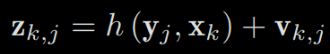
Assuming an observation of the road sign yj at xk, corresponding to the pixel position on the image zk,j , then, the observation equation can be expressed as:

where K is the intrinsic matrix of the camera, and s is the distance of pixels, which is also the third element of (Rkyj +tk). If we use transformation matrix Tk to describe the pose, then the points yj must be described in homogeneous coordinates, and then converted to non-homogeneous coordinates afterwards.

Now, consider what happens when the data is affected by noise. In the motion and observation equations, we usually assume that the two noise terms wk, vk,j satisfy a Gaussian distribution with zero mean, like this:

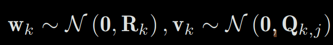
where N means Gaussian distribution, 0 means zero mean, and Rk, Qk,j is the covariance matrix. Under the influence of these noises, we hope to infer the pose x and the map y from the noisy data z and u (and their probability density distribution), which constitutes a state estimation problem.

Generally, there are two ways to deal with this state estimation problem. Since these data come gradually over time in the SLAM process, we should intuitively hold an estimated state at the current moment and then update it with new data. This method is called the incremental method, or filtering.

For a long time in history, researchers have used filters, especially the extended Kalman filter (EKF) and its derivatives, to solve it. The other way is to record the data into a file and looking for the best trajectory and map in all time. This method is called the batch estimation. In other words, we can collect all the input and observation data from time 0 to k together and ask, with such input and observation, how to estimate the entire trajectory and map from time 0 to k?

The incremental method only cares about the state estimation of the current moment xk but does not consider much about the previous state. Conversely, the batch method can be used to get an optimized trajectory in a long time, which is considered superior to the traditional filters and has become the mainstream method of current visual SLAM.

In SLAM, practical methods need to be real-time so have some compromises. For example, we fix some historical trajectories and only optimize some trajectories close to the current moment, leading to the sliding window estimation method described later.

To estimation the conditional pdf, we use the Bayes equation to switch the variables:

The left side is called posterior probability, and P(z|x) on the right is called likelihood (or likehood), and the other part is P(x) is called prior. It is normally difficult to find the posterior distribution directly (in nonlinear systems), but it is feasible to find an optimal point which maximize the posterior (Maximize a Posterior, MAP):

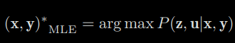
Please note that the denominator part of Bayes’ rule has nothing to do with the state x, y to be estimated, so it can be just ignored. Bayes’ rule tells us that solving the maximum posterior probability is equivalent to the estimate the product of maximum likelihood and a priori. Further, we can also say, “I’m sorry, I don’t know in prior where the robot pose or the map points are”, then there is no prior. In this case, we can solve the Maximize Likelihood Estimation (MLE):

3-1-2) Introduction to Least-squares

Now we have formulated the state estimation problem into a MAP/MLE problem, and the next question is how to solve it. Under the assumption of Gaussian distribution, we can have a simpler form of the maximum likelihood problem. Looking back at the observation model, for a certain kind of observation, we have:

Since we assume the noise item is Gaussian, which means vk ∼ N (0, Qk,j ), so the conditional probability of the observation data is:

which is, of course, still a Gaussian distribution. Now let’s consider solving the maximum likelihood estimation under this single observation.

After some simplification described in the book, we find that the least-squares problem in SLAM has some specific structures: First, the objective function of the whole problem consists of many (weighted)

• First, the objective function of the whole problem consists of many (weighted) error quadratic forms. Although the overall state variable’s dimensionality is very high, each error term is simple and is only related to one or two state variables. For example, the motion error is only related to xk−1, xk, and the observation error is only related to xk, yj . This relationship will give a sparse least-square problem, which we will investigate further in the backend chapter.
• Secondly, if you use Lie algebra to represent the increment, the problem is the least-squares problem of unconstrained. However, if the rotation matrix/transformation matrix is used to describe the pose, the constraint of the rotation matrix itself will be introduced, that is, “s.t. RT R = I and det(R) = 1 ” need to be added to the problem. Additional constraints can make optimization more difficult
• Finally, we used a quadratic metric error, exactly the L2−norm. The information matrix is used as the weights of each element. For example, if an observation is very accurate, the covariance matrix will be “small” and the information matrix will be “large”, so this error term will have a higher weight than the others in the whole problem. We will see some drawbacks of the L2 error later.

Next, we will introduce how to solve this least-squares problem, which requires some basic knowledge of nonlinear optimization. In particular, we want to discuss how to solve such a general unconstrained nonlinear least-squares problem.

3-2) Nonlinear Least-square Problem

For a given equation, let

the derivative of the objective function be zero, and then find the optimal value of x, just like finding the extreme value of a scalar function. If f is just a simple linear function, then the problem is only a simple linear least-square problem. But, some derivative functions may be complicated in form, making the equation difficult to solve. Solving this equation requires us to know the global property of the objective function, which is usually not possible. For the least-square problem that is inconvenient to solve directly, we can use the iterated methods to start from an initial value and continuously update the current estimations to reduce the objective function. The specific steps can be listed as follows:

• Give an initial value x0
• For k-th iteration, we find an incremental value of ∆xk, such that the object function norm2(kf(xk + ∆xk)k) reaches a smaller value
• If ∆xk is small enough, stop the algorithm
• Otherwise, let xk+1 = xk + ∆xk and return to step 2

When the function decreases until the increment becomes very small, it is considered that the algorithm converges, and the objective function reaches a minimum value. In this process, the problem is how to find the increment at each iteration point, which is a local problem. We only need to be concerned about the local properties of f at the iteration value rather than the global properties. Such methods are widely used in optimization, machine learning, and other fields.

Next, we examine how to find this increment ∆xk. This part of knowledge belongs to the field of numerical optimization.

3-2-1) The First and Second-order Method

Now consider the k-th iteration. Suppose we are at xk and want to find the increment ∆xk, then the most intuitive way is to make the Taylor expansion of the objective function in xk:

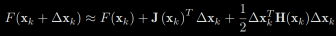
where J(xk) is the first derivative of F(x) with respect to x (also called gradient, Jacobi Matrix, or Jacobian), H is the second-order derivative (or Hessian), which are all taken at xk.

We can choose to keep the first-order or secondorder terms of the Taylor expansion, and the corresponding solution is called the first-order or the second-order method. In the simplest way, if we only keep the firstorder one, then taking the increment at the minus gradient direction will ensure that the function decreases.

Usually, we have to compute another step length parameter, say, λ. The step length can be calculated according to certain conditions.

The first-order and second-order methods are very intuitive, as long as we can calculate the Taylor expansion of f and find the increments.

3-2-2) The Gauss-Newton Method

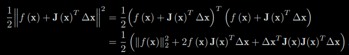
The Gauss-Newton method is one of the simplest methods in optimization algorithms. Its idea is to carry out a first order Taylor expansion of f(x). According to the extreme conditions, this time we set the derivative with ∆x to zero to reach the extreme value. To do this, let’s first expand the square term of the objective function:

We find the derivative of the above formula with respect to ∆x and set it to zero. The following equation can be obtained:

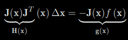
We define the coefficients on the left as H and the coefficient on the right as g, then the above formula becomes:
H∆x = g. If we can get the ∆x in each iteration, then the algorithm of the Gauss-Newton method can be written as:

• Set it initial value as x0
• For k-th iteration, calculate the Jacobian J(xk) and residual f(xk)
• Solve the normal equation: H∆xk = g
• If ∆xk is small enough, stop the algorithm. Otherwise let xk+1 = xk+∆xk and return to step 2

3-2-3) The Levernberg-Marquatdt Method

The approximate second-order Taylor expansion used in the Gauss-Newton method can only have a good approximation effect near the expansion point. So, we naturally thought a range should be added to ∆x, called trust-region. This range defines under what circumstances the second-order approximation is valid. This type of method is also called trust-region method. We think the approximation is valid only in the trusted region; otherwise, it may go wrong if the approximation goes outside.

So how to determine the scope of this trust-region? A good method is to determine it based on the difference between our approximate model and the real object function: if the difference is small, it means that the approximation is good, and we may expand the trust-region; conversely, if the difference is large, we will reduce the range of approximation. We define an indicator ρ to describe the degree of approximation:

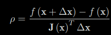
The numerator of ρ is the decreasing value of the real object function, and the denominator is the decreasing value of the approximate model. If ρ is close to 1, we may say the approximation is good. A small ρ is indicating that the actual reduced value is far less than the approximate reduced value.

Therefore, we build an improved version of the nonlinear optimization framework, which will have a better effect than the Gauss-Newton method:

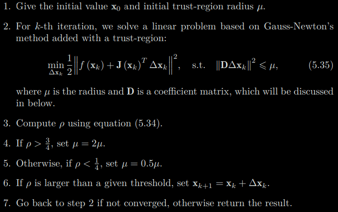
In the optimization method proposed by Levenberg, taking D into the unit matrix I is equivalent to directly constraining ∆xk in a sphere. Subsequently, Marquardt proposed to take D as a non-negative diagonal matrix. In practice, the square root of the diagonal elements of J T J is usually used as D so that the constraint range is larger on the dimensions with small gradient.

In any case, in Levenberg-Marquardt optimization, we need to solve a subproblem like (5.35) to obtain the gradient. This sub-problem is an optimization problem with inequality constraints. We use Lagrangian multipliers to put the constraints in the objective function to form the Lagrangian function:

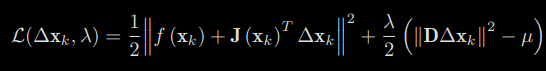
where λ is the Lagrange multiplier. Similar to the method in the Gauss-Newton, let the derivative of the Lagrangian function with respect to ∆x be zero, and we still need to solve the linear equation for calculating the increment.

It can be seen that the incremental equation has an extra λDT D compared to the Gauss-Newton method. If you consider its simplified form D = I, then it is equivalent to solving: (H + λI) ∆xk = g.

In practice, there are also many other ways to solve the increment, such as DogLeg and other methods. What we have introduced here is just the most common and basic method, and it is also the most widely-used method in visual SLAM. We usually choose one of the Gauss-Newton or Levenberg-Marquardt methods as the gradient descent strategy in practical problems. When the problem is well-formed, Gauss-Newton is used. Otherwise, in ill-formed problems, we use the LevenbergMarquardt method.

4) Conclusion

I hope that the summary of the theoretical part of this book can help some people. I wrote it as I took notes in order to keep what I found important for an overall understanding. Of course, if a very precise understanding is needed, I can only recommend reading the book directly.