

Unveiling Earth’s Secrets: A Guide to Deep Learning Applications in Satellite-Based Land Cover Classification (1/4)
Part 1/4: Google Earth Engine to build a dataset with satellite images
This article explains how to get satellite images to build a dataset to train a neural network. It will first explain the MiniFrance land cover dataset, details about satellite data (TIF files, EPSG projections, etc.), and how to visualize data on Google Maps through the QGIS software. Then, a description of the two satellites used Sentinel 1 and Sentinel 2 will be given. Finally, we will go deeper into the code implementation to fetch satellite images using Google Earth Engine.
The code can be found here.
Table of contents
- Introduction
- MiniFrance land cover dataset
- Dataset overview
- Tif files
- Definition
- Characteristics
- How to visualize satellite data in QGIS
- Satellite images
- Sentinel 2 (optical)
- Multispectral Imaging
- Global Coverage
- High Resolution
- Open Data Policy
- Sentinel 1 (SAR)
- Synthetic Aperture Radar (SAR)
- Dual-Polarization
- VV-VH polarizations
- Ground Type Differentiation
- Interferometric Capabilities
- Global Coverage
- Satellites overview
- EPSG Projections
- Satellites overview
- Sentinel 2 (optical)
- Google Earth Engine
- Overview
- Petabyte-Scale Data Archive
- Cloud Computing Infrastructure
- Time-Series Analysis
- Integration of Remote Sensing Algorithms
- Project setup
- Implementation
- Fetch GEE image on specific area
- Filter result
- Manage projection to align sat images with targets
- Visualizing results
- Sentinel 1 VV and VH polarizations
- Sentinel 2 data
- Overview
- Conclusion
1) Introduction
In an era marked by unprecedented technological advancements, our ability to understand and monitor the Earth has taken giant leaps forward. Satellites, orbiting high above the planet, have become indispensable tools in unraveling the intricacies of our dynamic planet. The data they provide has far-reaching implications for a variety of fields, from climate science to urban planning.
One particular aspect of satellite-based studies gaining prominence is the extraction of valuable information from images for land cover analysis. Land cover, encompassing natural landscapes and man-made features, is a fundamental component of Earth’s surface. Building datasets for land cover tasks using satellite images is an approach that allows us to categorize and understand the diverse types of terrain that make up our planet. In the following sections, we will explore the intricacies of constructing datasets for land cover analysis, shedding light on the methodologies and tools that enable us to glean meaningful insights from the vast troves of satellite imagery.
At the end of this article, readers will have a better understanding of how to manipulate satellite images, both with a tool and by programming. This learning will be done by studying a practical case of creating a Land Cover database which will be used to train a neural network.
2) MiniFrance land cover dataset
Dataset link: https://ieee-dataport.org/open-access/minifrance
2-1) Dataset overview
Description from the authors:
“We introduce a novel large-scale dataset for semi-supervised semantic segmentation in Earth Observation: the MiniFrance suite.
MiniFrance has several unprecedented properties: it is large-scale, containing over 2000 very high resolution aerial images,; it is varied, covering 16 conurbations in France, with various climates, different landscapes, and urban as well as countryside scenes; and it is challenging, considering land use classes with high-level semantics. Nevertheless, the most distinctive quality of MiniFrance is being the only dataset in the field especially designed for semi-supervised learning: it contains labeled and unlabeled images in its training partition, which reproduces a life-like scenario.”
List of annotated classes:
0: No information
1: Urban fabric
2: Industrial, commercial, public, military, private and transport units
3: Mine, dump and contruction sites
4: Artificial non-agricultural vegetated areas
5: Arable land (annual crops)
6: Permanent crops
7: Pastures
8: Complex and mixed cultivation patterns
9: Orchards at the fringe of urban classes
10: Forests
11: Herbaceous vegetation associations
12: Open spaces with little or no vegetation
13: Wetlands
14: Water
15: Clouds and shadows
The labels are provided in TIF files, which is much appreciated as this will allow us to know the exact location of each label to download the satellite images of our choice. The next section will explains what are TIF files.
2-2) Tif files
Remote sensing plays a crucial role in acquiring information about the Earth’s surface from a distance, and the data obtained is often stored in various file formats. One such important format frequently used in remote sensing is the Tagged Image File Format (TIF). In this chapter, we will explore what TIF files are, their characteristics, and why they are widely employed in the field of remote sensing.
2-2-1) Definition
TIF, or TIFF, stands for Tagged Image File Format. It is a popular and versatile file format used for storing images, including those generated by remote sensing instruments. TIF files can store both raster and vector data, making them suitable for a wide range of applications.
2-2-2) Characteristics
- Lossless Compression: TIF files typically use lossless compression, meaning that the image quality remains intact without any loss of information. This is crucial in remote sensing applications where high precision is essential.
- Metadata: TIF files support the inclusion of metadata, which provides additional information about the image. This metadata can include details such as sensor information, acquisition date, and geographic coordinates, enhancing the interpretability of the data.
- Multi-channel Support: Remote sensing often involves the acquisition of data in multiple spectral bands. TIF files can store multi-channel or multispectral data efficiently, making them suitable for representing complex information captured by various sensors.
- Georeferencing: TIF files can be georeferenced, allowing the spatial information within the image to be associated with specific geographic locations. This is essential for accurate mapping and analysis in remote sensing applications.
Understanding the fundamentals of TIF files is essential for remote sensing engineers and researchers. The format’s lossless compression, support for metadata, multispectral capabilities, and georeferencing make it a preferred choice for storing and analyzing the wealth of information acquired through remote sensing technologies.
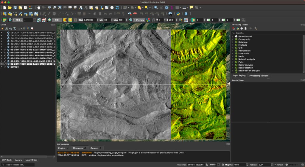
2-3) How to visualize satellite data in QGIS
QGIS, which stands for Quantum GIS, is an open-source Geographic Information System (GIS) software that provides a powerful platform for viewing, analyzing, and managing spatial data. Developed by a community of volunteers and supported by the Open Source Geospatial Foundation (OSGeo), QGIS is freely available and widely used by professionals, researchers, and enthusiasts in the field of geospatial technology.
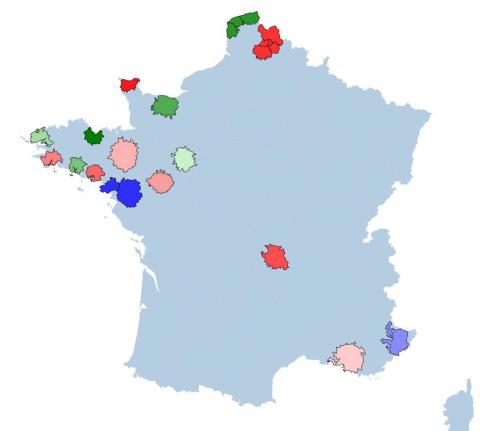
Once the MiniFrance dataset is downloaded, the labeled data containing the 16 classes can be open in QGIS:
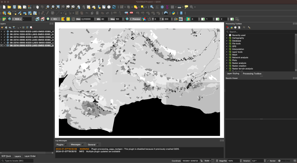
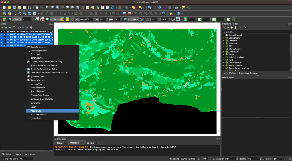
By default for one-channel data, QGIS will apply a grayscale colormap. This can be changed by double clicking on one sample, to apply a random of chosen color:
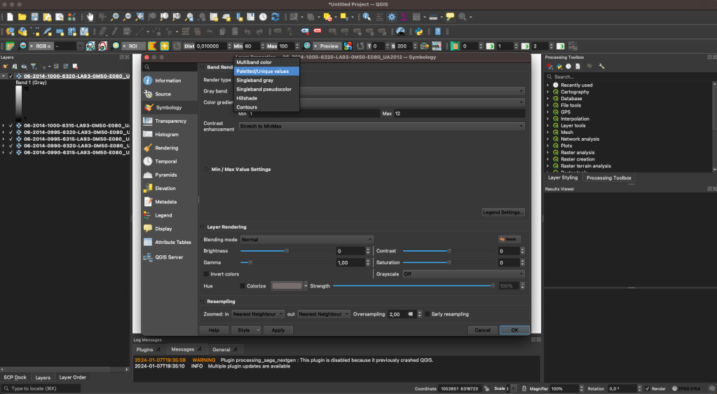


Then, this colormap, called a Style, can be copy-paste to all other data:
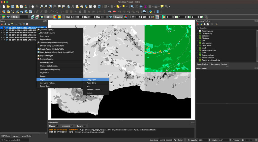
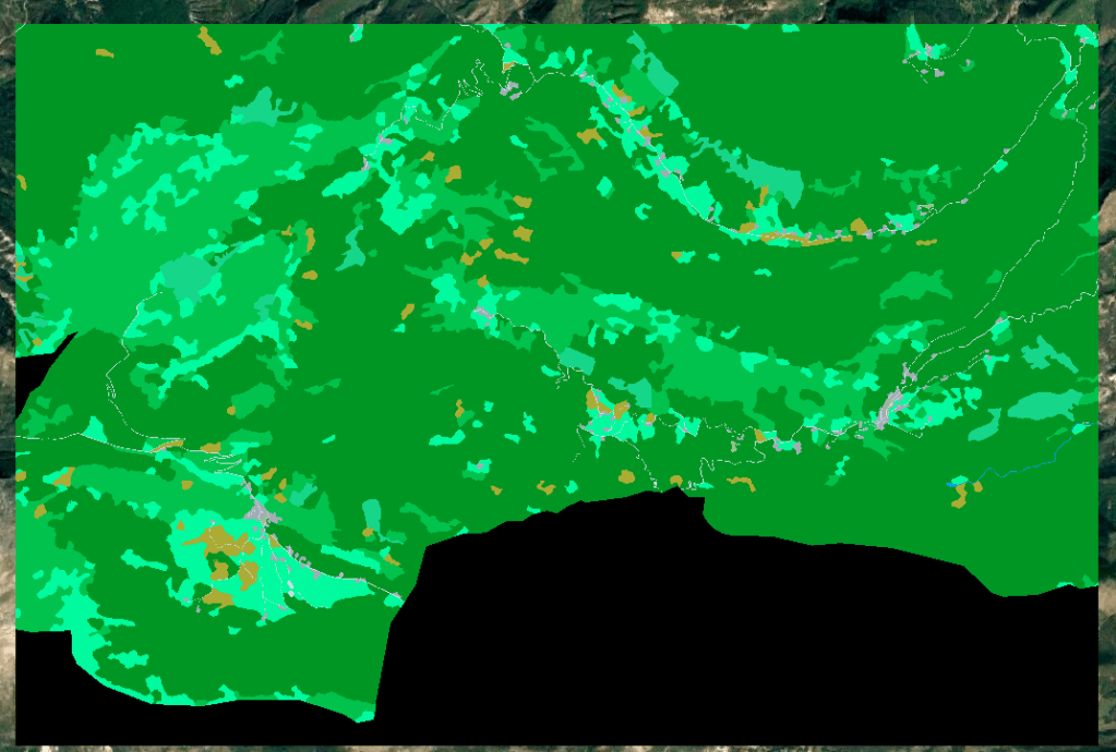
A useful feature is to add a Google Maps view (or other provider) to see what the ground looks like. To do so, first click on the red rectangle, then on the blue one and fill in the information:
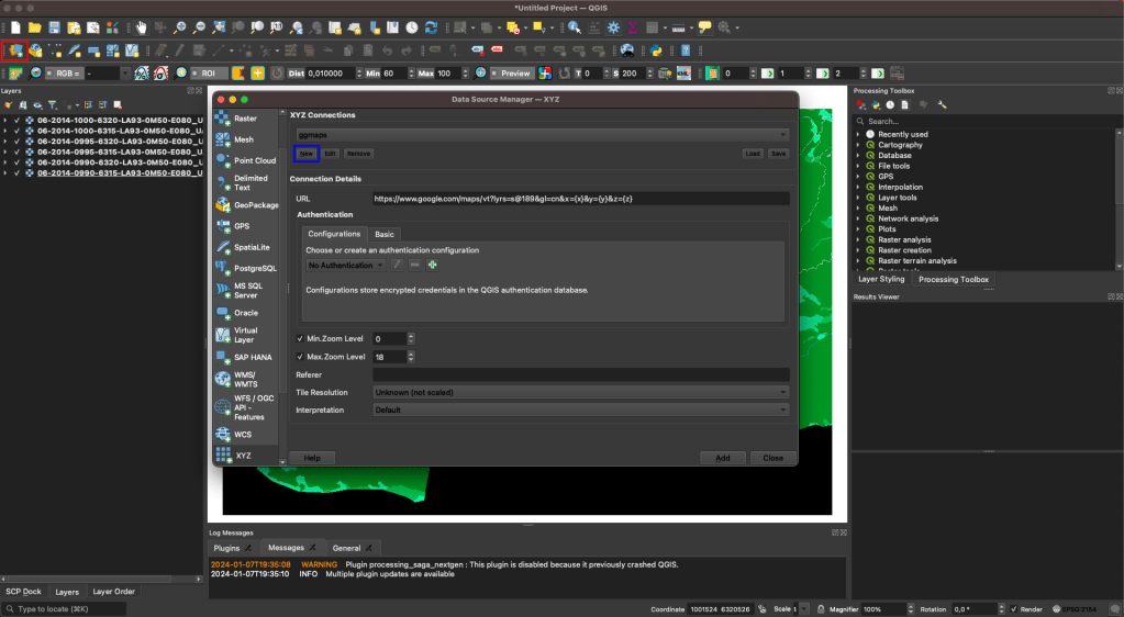
Then, Google maps will be displayed as a new layer:

3) Satellite images
3-1) Sentinel 2 (optical)
Meet Sentinel-2, a star player in the realm of remote sensing and Earth observation. This section will guide you through the intricacies of this remarkable satellite, explaining how it revolutionizes our understanding of Earth’s dynamics.
Sentinel-2, part of the European Space Agency’s Copernicus program, represents a pinnacle in satellite technology dedicated to monitoring the Earth’s surface with unprecedented detail. Launched with the primary objective of providing timely and high-resolution imagery for a range of applications, Sentinel-2 has become an indispensable tool for researchers, environmentalists, and policymakers alike.
3-1-1) Multispectral Imaging
One of the standout features of Sentinel-2 is its multispectral imaging capabilities. Equipped with a powerful multispectral instrument, this satellite captures imagery in thirteen spectral bands, ranging from visible to shortwave infrared. This wealth of spectral information enables us to distinguish and analyze various surface features with unparalleled precision.
Sentinel-2 Bands:
1. Visible and Near-Infrared (VNIR) Bands:
- Band 1 (Coastal Aerosol – 443 nm): This band is sensitive to the presence of aerosols and other particles in coastal waters.
- Band 2 (Blue – 490 nm): Captures blue light, useful for vegetation studies and water quality assessments.
- Band 3 (Green – 560 nm): Represents green light and is particularly useful for monitoring vegetation health.
- Band 4 (Red – 665 nm): This band is sensitive to red light and is essential for vegetation analysis, including assessing plant vitality.
2. Red-Edge and Near-Infrared (NIR) Bands:
- Band 5 (Red Edge 1 – 705 nm): This band is positioned in the red-edge portion of the spectrum, which is sensitive to changes in chlorophyll content in plants.
- Band 6 (Red Edge 2 – 740 nm): Similar to Band 5, this band provides information on plant health and stress.
- Band 7 (Red Edge 3 – 783 nm): Another red-edge band for vegetation monitoring.
- Band 8A (NIR – 865 nm): Captures near-infrared light and is crucial for vegetation health assessment, including the calculation of vegetation indices.
3. Shortwave Infrared (SWIR) Bands:
- Band 8 (SWIR 1 – 945 nm): The first shortwave infrared band, sensitive to changes in vegetation structure and moisture content.
- Band 9 (SWIR 2 – 1375 nm): This band is useful for assessing water content in vegetation and soil.
- Band 10 (SWIR 3 – 1610 nm): Captures additional information on vegetation moisture and other surface features.
- Band 11 (SWIR 4 – 2190 nm): The longest wavelength in the SWIR range, providing information on moisture and geological features.
4. Cirrus and Thermal Infrared Bands:
- Band 12 (SWIR 5 – 2290 nm): This band is sensitive to atmospheric cirrus clouds, aiding in cloud detection and removal.
- Band 13 (SWIR 6 – 3740 nm): Captures thermal infrared radiation, allowing for the estimation of land surface temperature.
- Band 14 (SWIR 7 – 3910 nm): Another thermal infrared band for land surface temperature estimation.
Specific combinations of these bands are used in function of the domain application. These combinations can be done in RGB of single-gray band as a formula. For instance, to study vegetation, a common index is the NDVI (normalized difference of the red and the infrared band), calculated as NDVI = (NIR-RED) / (NIR+RED).
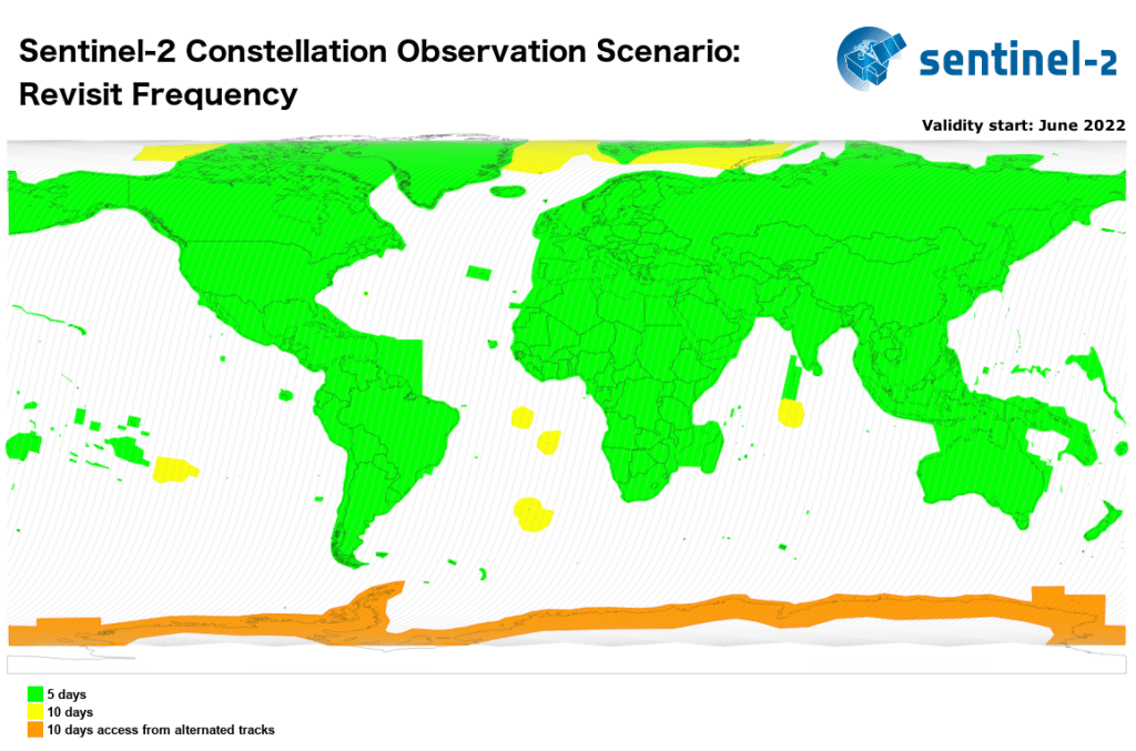
3-1-2) Global Coverage
Sentinel-2 operates on a systematic and global acquisition strategy. Every five days, it captures imagery of the entire Earth’s land surface, ensuring a frequent revisit time that is crucial for monitoring dynamic changes such as vegetation growth, land use alterations, and natural disasters.
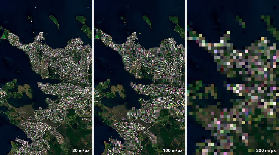
3-1-3) High Resolution
The satellite boasts a spatial resolution ranging from 10 to 60 meters per pixel, allowing us to discern fine details on the Earth’s surface. This level of detail is particularly advantageous for applications such as agricultural monitoring, forestry management, and urban planning.
3-1-4) Open Data Policy
In a move towards fostering global collaboration and knowledge sharing, Sentinel-2 follows an open data policy. This means that the acquired imagery is freely accessible to the public, promoting a democratic approach to Earth observation data and encouraging a wide array of applications and research.
Sentinel-2’s capabilities extend across a spectrum of applications. From precision agriculture and forestry management to disaster monitoring and urban planning, the satellite’s data proves instrumental in addressing critical challenges that our planet faces today.
3-2) Sentinel 1 (SAR)
Meet Sentinel-1, a sentinel from the European Space Agency’s Copernicus program, armed with an advanced synthetic aperture radar (SAR) system. Here are the features and capabilities of Sentinel-1:
3-2-1) Synthetic Aperture Radar (SAR)
At the heart of Sentinel-1 lies its Synthetic Aperture Radar, a revolutionary technology that transcends the limitations of traditional optical sensors. Unlike optical satellites that rely on sunlight to capture images, SAR operates day and night, in all weather conditions. By emitting microwave pulses and measuring the reflections, Sentinel-1 penetrates through clouds, rain, and darkness to provide an unobstructed view of the Earth’s surface.
3-2-2) Dual-Polarization
Sentinel-1 boasts dual-polarization capabilities, capturing data in both horizontal and vertical polarizations. This dual-polarization feature enhances the interpretability of the acquired imagery, enabling scientists and engineers to discern subtle variations in surface properties.

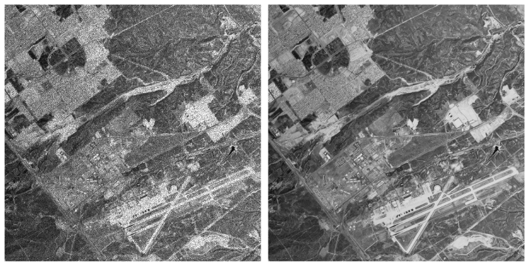
As VV and VH will be the ones we will used, we will go deeper into these two polarisations.
These images have a lot of noise called Speckle which needs to be filter. One common technique is to average multiple images temporally. Example:
3-2-2-1) VV-VH polarizations
– VV Polarization:
VV polarization refers to the transmission and reception of radar signals in the vertical plane. In this configuration, both the transmitting and receiving antennas have their polarization aligned vertically.
VV polarization is sensitive to the vertical structure of the target and is particularly effective at highlighting surface roughness and vegetation.
– VH Polarization:
VH polarization involves transmitting the radar signal in the vertical plane and receiving it in the horizontal plane. The transmitting antenna has a vertical polarization, while the receiving antenna has a horizontal polarization.
VH polarization is sensitive to structures with a combination of vertical and horizontal features, making it useful for discriminating between different ground types based on their geometric properties.
3-2-2-2) Ground Type Differentiation
- Urban Areas:
- VV polarization is effective in urban areas as it highlights the vertical structures of buildings and infrastructure. This polarization is suitable for identifying built-up areas and analyzing urban development patterns.
- VH polarization, on the other hand, can provide additional information on the orientation and surface roughness of structures. It is beneficial in discriminating between different building materials and construction types within urban environments.
- Vegetation:
- VV polarization is sensitive to the vertical structure of vegetation, making it valuable for monitoring forests and assessing vegetation health. It penetrates through the canopy and provides information on the density and structure of vegetation.
- VH polarization is also useful for vegetation analysis, especially in areas with dense vegetation cover. It captures information related to the scattering properties of leaves and branches, aiding in the discrimination of different vegetation types.
- Agricultural Land:
- In agricultural areas, VV polarization can be effective in characterizing crop types and monitoring crop growth stages. It is sensitive to the surface roughness of the soil and can provide insights into soil moisture conditions.
- VH polarization is valuable for distinguishing between different types of crops based on their orientation and canopy structure. It can also aid in assessing soil moisture content and surface roughness variations.
We will see examples of VV and VH data in the last section on Google Earth Engine.
3-2-3) Interferometric Capabilities
Sentinel-1 is equipped with interferometric capabilities, allowing for the generation of interferograms. This technology enables precise measurements of ground deformation, making it an invaluable tool for monitoring earthquakes, subsidence, and other geophysical phenomena.
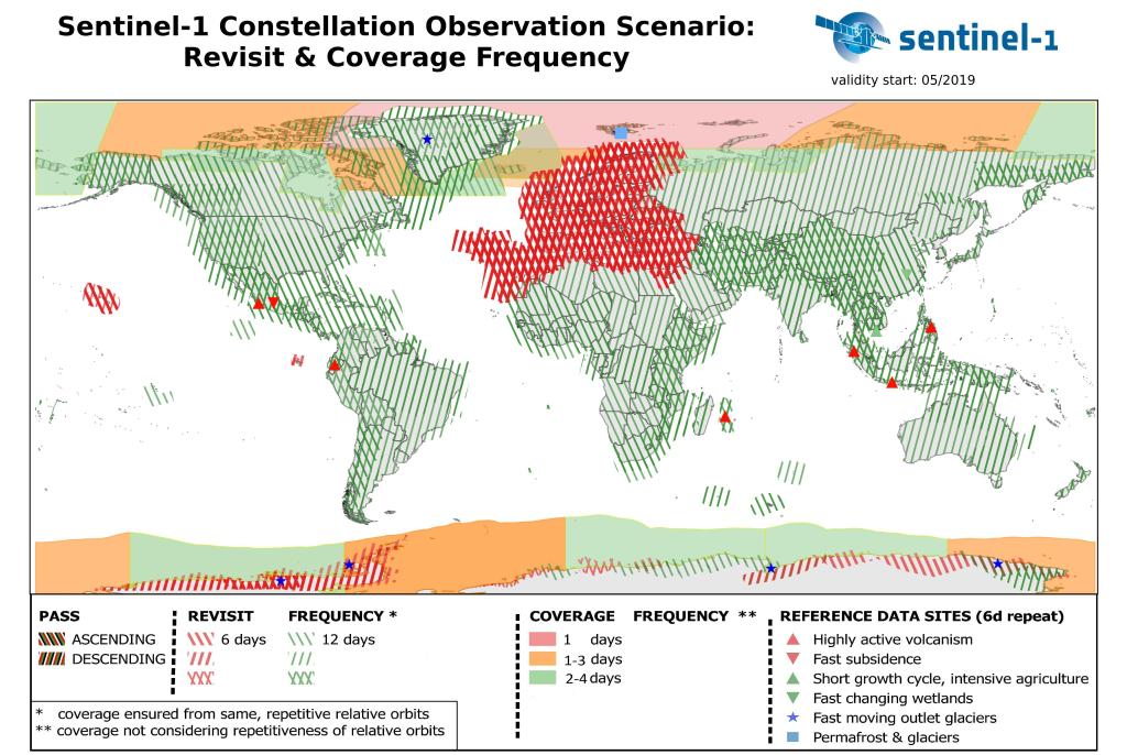
3-2-4) Global Coverage
Similar to its counterpart Sentinel-2, Sentinel-1 operates on a systematic acquisition strategy, providing global coverage at regular intervals. This systematic revisit allows for continuous monitoring of dynamic Earth processes, making it an essential asset for applications ranging from environmental monitoring to disaster response.
Sentinel-1’s versatility opens doors to a multitude of applications across various domains. From monitoring ground displacement and subsidence to mapping changes in land cover and detecting oil spills at sea, the satellite’s SAR imagery serves as an invaluable resource for understanding the Earth’s dynamic processes.
3-3) EPSG Projections
Understanding the concept of EPSG projections is crucial for anyone working with geospatial data. EPSG refers to the European Petroleum Survey Group, which created a database of coordinate reference systems and transformations. These systems, known as EPSG codes, help standardize the way we represent spatial information on maps and satellite images.
EPSG projections, or EPSG codes, are numerical identifiers assigned to coordinate reference systems (CRS) and coordinate transformations. These codes provide a standardized way to define the spatial characteristics of a dataset, ensuring consistency in how geographic information is represented and interpreted.
Key Components:
- Coordinate Reference System (CRS):
- A CRS defines how locations on the Earth’s surface are represented using coordinates. It includes parameters such as the coordinate system, map projection, and datum.
- EPSG Code:
- The EPSG code uniquely identifies a specific CRS or transformation in the EPSG database. For example, EPSG:4326 represents the WGS 84 coordinate system commonly used for representing latitude and longitude.
Examples of EPSG Projections:
1. WGS 84 (EPSG:4326):
- The most commonly used EPSG projection is WGS 84 (World Geodetic System 1984). It uses a geographic coordinate system with latitude and longitude. For example:
- Latitude: 34.0522° N, Longitude: -118.2437° W
2. UTM (Universal Transverse Mercator) Zones (EPSG:326XX):
- UTM divides the world into zones, each with its own projection. For instance, UTM Zone 33N is represented by EPSG:32633. Example coordinates:
- Easting: 500000 meters, Northing: 4649776 meters
3. Web Mercator (EPSG:3857):
- Web Mercator is used for online mapping services like Google Maps. It’s based on a pseudo-mercator projection suitable for web applications. Example coordinates:
- X: 13962633 meters, Y: 826918.67 meters
4. Albers Equal Area Conic (EPSG:102003):
- Albers Equal Area Conic is used to represent large areas with minimal distortion. Example coordinates:
- False Easting: 0 meters, False Northing: 0 meters
Importance in Satellite Image Analysis:
- Consistency:
- Using EPSG codes ensures consistency in spatial representations across different datasets and software platforms. This is crucial for accurate analysis and integration of diverse geospatial data sources, including satellite images.
- Coordinate Transformation:
- EPSG codes facilitate seamless coordinate transformations between different reference systems. This is essential when working with satellite imagery from different sensors or missions that might use different coordinate systems.
- Interoperability:
- As a remote sensing engineer, understanding EPSG codes promotes interoperability, allowing you to combine datasets from various sources and apply consistent spatial analysis techniques across your projects.
- Web Mapping:
- Many web mapping services use EPSG codes to define the coordinate systems for displaying satellite imagery and maps online. Understanding and specifying the correct EPSG code is crucial when integrating satellite data into web applications.
In summary, EPSG projections play a vital role in remote sensing and satellite image analysis by providing a standardized way to represent and manage spatial information. They ensure consistency, enable interoperability, and facilitate accurate spatial analysis in diverse geospatial applications.
3-4) Satellites overview
Here’s an overview of some commonly used satellite systems and their applications in remote sensing:
- Landsat Series:
- Key Characteristics: Landsat satellites capture multispectral imagery in visible, near-infrared, and thermal bands.
- Applications: Land cover classification, vegetation monitoring, agriculture assessment, and change detection.
- Sentinel Series (Sentinel-1 and Sentinel-2):
- Sentinel-1:
- Key Characteristics: Synthetic Aperture Radar (SAR) satellite, operates day and night, all-weather capability.
- Applications: Land deformation monitoring, disaster response, and ice monitoring.
- Sentinel-2:
- Key Characteristics: Multispectral imagery with high spatial resolution.
- Applications: Land cover mapping, crop monitoring, forest management, and environmental monitoring.
- Sentinel-1:
- MODIS (Moderate Resolution Imaging Spectroradiometer):
- Key Characteristics: Moderate spatial resolution with daily global coverage.
- Applications: Climate monitoring, land cover mapping, and monitoring vegetation health.
- ASTER (Advanced Spaceborne Thermal Emission and Reflection Radiometer):
- Key Characteristics: Captures data in multiple spectral bands, including thermal infrared.
- Applications: Land surface temperature estimation, geological mapping, and urban planning.
- WorldView Series (WorldView-2, WorldView-3):
- Key Characteristics: High spatial resolution, panchromatic and multispectral imagery.
- Applications: Urban planning, disaster response, agriculture, and natural resource management.
- RADARSAT Series (RADARSAT-2):
- Key Characteristics: Synthetic Aperture Radar (SAR) satellite.
- Applications: Ice monitoring, agriculture, forestry, and oil spill detection.
- GOES (Geostationary Operational Environmental Satellite):
- Key Characteristics: Geostationary orbit, continuous monitoring of a fixed area.
- Applications: Weather monitoring, atmospheric studies, and disaster monitoring.
- TerraSAR-X:
- Key Characteristics: Synthetic Aperture Radar (SAR) satellite with high spatial resolution.
- Applications: Terrain mapping, land cover classification, and disaster monitoring.
- Suomi NPP (National Polar-orbiting Partnership):
- Key Characteristics: Polar-orbiting satellite, collects data for climate research and weather forecasting.
- Applications: Climate monitoring, atmospheric studies, and global temperature measurements.
- Copernicus Sentinel-3:
- Key Characteristics: Ocean and land monitoring satellite with multiple instruments.
- Applications: Oceanography, sea surface temperature monitoring, land surface temperature monitoring.
This list is not exhaustive.
4) Google Earth Engine
4-1) Overview
Many tutorials are available on the Google developers website.
This powerful tool transcends traditional boundaries, enabling researchers and scientists to unlock the vast potential of Earth observation data. In this chapter, we will delve into the intricacies of Google Earth Engine, examining its unique features and the transformative impact it has on our ability to analyze and understand our planet.
4-1-1) Petabyte-Scale Data Archive
At the core of Google Earth Engine is a vast archive of Earth observation data, reaching petabyte-scale. This includes a diverse array of satellite imagery, climate data, and geospatial datasets from various sources. This massive data repository is instantly accessible, providing researchers with a wealth of information to analyze and interpret Earth’s dynamic processes.
4-1-2) Cloud Computing Infrastructure
Leveraging the power of cloud computing, Google Earth Engine enables seamless analysis of large-scale geospatial data. The platform harnesses the computing muscle of Google’s infrastructure, allowing users to process, visualize, and derive insights from massive datasets without the need for extensive computing resources on local machines.
4-1-3) Time-Series Analysis
One of the standout features of Google Earth Engine is its ability to perform time-series analysis on Earth observation data. This temporal dimension allows researchers to track changes over time, monitor trends, and gain a deeper understanding of dynamic processes such as deforestation, urbanization, and climate change.
4-1-4) Integration of Remote Sensing Algorithms
Google Earth Engine provides an extensive library of pre-built remote sensing algorithms, simplifying the implementation of complex analyses. This empowers users with varying levels of expertise to apply advanced techniques for land cover classification, vegetation monitoring, and other geospatial analyses.
4-2) Project setup
On the official starting page, follow the Getting Access steps to sign up and create a Google Earth Engine project. The name of the project will be needed for initialisation to let you access satellite images. Once the setup is done, the authentication should works by running the next command in a terminal:
earthengine authenticate
Once the earthengine-api is installed:
pip install earthengine authenticate
The next python code should run (“gee_project_name” should be replaced by the user’s project name created during the Getting Access steps.
import ee
ee.Initialize(project=gee_project_name)
4-3) Implementation
The objectif for building our dataset to train a neural network is to get its inputs and its targets. The targets come from the MiniFrance dataset described earlier, and the inputs should be Sentinel 1 and Sentinel 2 images (or other satellites but we choose these 2 as example for this project). Theses images are available in Google-Earth-Engine through datasets. For the next sections we will only take as example the use of Sentinel 1 images, but the code for both Sentinel 1 and Sentinel 2 are available on the Github repository.
4-3-1) Fetch GEE image on specific area
Once GEE is installed, we can access to images collections of specific satellites. Here is the Sentinel 1 example:
dataset = ee.ImageCollection("COPERNICUS/S1_GRD")
Please note that we use the “_GRD” which is an already preprocessed S1 image source.
This dataset object is a link to all S1 images world-wide since the satellite release. What we need is images corresponding to one label data on the good date (each label file has year in its filename). After extracting the year of the first label, we will convert it to a GeoSerie to extract the shape of the TIF file. This GeoSerie will be used by GEE to crop the dataset to the target area:
# read tif file to extract coordinates
with rasterio.open(label_path) as label_raster:
    box_raster = box(label_raster.bounds.left, label_raster.bounds.bottom, label_raster.bounds.right, label_raster.bounds.top)
    geo_series = GeoSeries([box_raster], crs=label_raster.crs)
coordinates = list(geo_series.to_crs("EPSG:4326").unary_union.envelope.exterior.coords)
geom = ee.Geometry.Polygon([coordinates])
feature = ee.Feature(geom, {})
aoi = feature.geometry()
Please note that the data from GEE is downloaded in “EPSG:4326” which will need a projection to fit our data.
4-3-2) Filter result
GEE has a good mechanism of filtering for any propertie. For each dataset, the list of its properties can be found on their documentation.
We will first filter on the shape, start and end date:
dataset = ee.ImageCollection("COPERNICUS/S1_GRD").filterBounds(aoi)
images_collection = dataset.filter(ee.Filter.eq("instrumentMode", "IW")).filterDate(start_date, end_date)
As mentioned in the first sections, we will want to reduce speckle by temporally averaging multiple images. To do this, we could retrieve all S1 images as of the annotation date (indicated in the file name). But this technique has a problem, it averages data having different views of the area. Indeed, the satellites can be in descending or ascending pass, and each orbit has a number. To reduce the speckle but without losing too much precision, the best is to average images with the same angle of incidence and therefore the same pass on the same orbit number.
# filter the results with the most present orbit sens
orbit_sens_list, counts = np.unique(
    images_collection.aggregate_array("orbitProperties_pass").getInfo(),
    return_counts=True,
)
indices = np.argsort(counts)
orbit_sens = orbit_sens_list[indices[-1]]
images_collection = images_collection.filter(ee.Filter.eq("orbitProperties_pass", orbit_sens))

# filter the results with the most present orbit number
orbit_numbers, counts = np.unique(
    images_collection.aggregate_array("relativeOrbitNumber_start").getInfo(),
    return_counts=True,
)
indices = np.argsort(counts)
orbit_number = int(orbit_numbers[indices[-1]])
images_collection = images_collection.filter(ee.Filter.eq("relativeOrbitNumber_start", orbit_number))
We will then fetch the VH and VV features and average them:
vh_collection = images_collection.select("VH")
vv_collection = images_collection.select("VV")

vh_image = ee.Image(vh_collection.mean())
vv_image = ee.Image(vv_collection.mean())
4-3-3) Manage projections to align sat images with targets
As mentioned previously with the “EPSG:4326“, these downloaded images as in a specific projection called 4326 (described in “EPSG Projections” section). However, the annotated TIF files from the MiniFrance dataset are in EPSG:2154 which is a projection specific to France.
The Rasterio package, which is a very usefull package for satellite data manipulation, has a specific function to do this projection called: reproject:
# reproject feature in 4326 to label crs
with rasterio.open(feature_path) as features_4326:
    t_transform, t_width, t_height = calculate_default_transform(features_4326.crs, label_crs, features_4326.width, features_4326.height, *features_4326.bounds)
    with rasterio.open(feature_path, "w", driver="GTiff", height=t_height, width=t_width, count=features_4326.count, dtype=features_4326.meta["dtype"], crs=label_crs, transform=t_transform) as dst:
        reproject(source=features_4326.read(), destination=rasterio.band(dst, 1), src_transform=features_4326.transform, src_crs=features_4326.crs, dst_transform=dst.transform, dst_crs=dst.crs)
Once the features VV and VH are reprojected to the good EPSG, we will need to crop the data to the label area:
# crop reprojected feature to the label shape
with rasterio.open(feature_path) as features_reprojected_raster:
    out_image, out_transform = mask(features_reprojected_raster, label_geo_series.geometry, crop=True)
    out_meta = features_reprojected_raster.meta.copy()

out_meta.update({"driver": "Gtiff", "height": out_image.shape[1], "width": out_image.shape[2], "transform": out_transform})

with rasterio.open(feature_path, "w", **out_meta) as dst:
    dst.write(out_image)
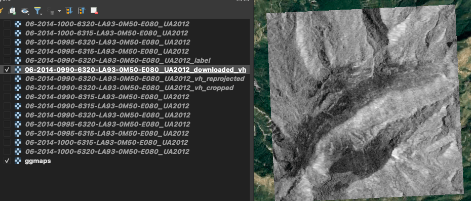
Illustrated steps where we can see:
- The labels, which is rectilinear as QGIS was open using the 2154 EPSG,
- Then an overlay of the labels on the downloaded VH polarization. We can notice that the polarization is not rectilinear as it is in another EPSG (4326),
- The downloaded polarization alone,
- The reprojected VH polarization, it is now rectilinear with white pixels added where data were missing,
- The cropped reprojected VH polarization which fit the labels


4-3-4) Visualizing results
Following the examples under the “How to visualize satellite data in QGIS” section, we can now visualize Sentinel 1 VV and VH polarization; and Sentinel 2 data.
4-3-4-1) Sentinel 1 VV and VH polarizations
The first column of 2 images are VV polarizations, the second column VH polarizations and the third one is an RGB composition of [VV, VH, None]:

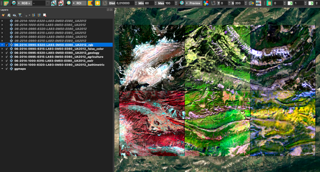
4-3-4-2) Sentinel 2 data
As Sentinel 2 has many bands (explained in the Sentinel 2 section), many RGB compositions can be down to show different ground characteristics. Sentinel-Hub website gives the most famous one here. Here are some examples:
6) Conclusion
In conclusion, the MiniFrance land cover dataset, with its comprehensive overview of Tif files, satellite images from Sentinel 2 (optical) and Sentinel 1 (SAR), provides a valuable resource for researchers and practitioners in the field of remote sensing and geospatial analysis. The dataset’s characteristics, including high resolution, global coverage, and open data policy, make it a versatile tool for various applications.
The utilization of Sentinel 2 optical imagery, with its multispectral imaging capabilities, allows for detailed land cover analysis. On the other hand, Sentinel 1 SAR data, with dual-polarization (VV-VH polarizations) and interferometric capabilities, enhances ground type differentiation, especially useful for applications such as agriculture and land deformation monitoring.
The article delves into the satellites’ overview, highlighting their EPSG projections and global coverage. Additionally, the integration of Google Earth Engine in the project setup showcases the platform’s capabilities in handling petabyte-scale data archives, utilizing cloud computing infrastructure for efficient processing, and enabling time-series analysis through the integration of remote sensing algorithms.
The implementation section outlines the steps to fetch Google Earth Engine images on a specific area, filter the results, and manage projections to align satellite images with targets. The article emphasizes the importance of proper visualization techniques, showcasing results from both Sentinel 1 VV and VH polarizations, as well as Sentinel 2 data.
As we continue to delve into the realm of remote sensing and geospatial exploration, your engagement is crucial. We encourage you to like and comment on this article, sharing your thoughts and insights. Your feedback contributes to a vibrant community of researchers and practitioners, fostering collaboration and pushing the boundaries of our understanding of Earth’s intricate landscapes.
